Economics Assignment: Managerial Decision Making and Economic Analysis
VerifiedAdded on 2020/04/07
|23
|4997
|33
Homework Assignment
AI Summary
This economics assignment provides a comprehensive analysis of managerial decision-making processes, emphasizing the importance of sound knowledge and proper reasoning in business contexts. It delves into the core elements of decision-making, including problem identification, solution development, and implementation, illustrated by the Woolworths case study. The assignment also explores marginal analysis as a crucial tool for optimizing profits, examining both linear and non-linear relationships in demand functions, and calculating elasticities. Furthermore, it investigates the concept of returns to scale in production, analyzing how changes in inputs affect output. The document includes detailed regression analyses, statistical interpretations, and practical applications of economic principles, offering a thorough understanding of key economic concepts and their practical implications in business decision-making.

Running head: ECONOMICS
Economics
Name of the Student
Name of the University
Author note
Economics
Name of the Student
Name of the University
Author note
Paraphrase This Document
Need a fresh take? Get an instant paraphrase of this document with our AI Paraphraser
1ECONOMICS
Table of Contents
Part 1................................................................................................................................................1
Answer 1......................................................................................................................................1
Answer 2......................................................................................................................................4
Part 2................................................................................................................................................5
Answer a......................................................................................................................................5
Answer b......................................................................................................................................7
Part 3................................................................................................................................................9
Answer a......................................................................................................................................9
Answer b....................................................................................................................................12
Part 4..............................................................................................................................................12
Answer a....................................................................................................................................12
Answer b....................................................................................................................................13
Answer c....................................................................................................................................14
Part 5..............................................................................................................................................15
Answer 1....................................................................................................................................15
Answer 2....................................................................................................................................18
Answer 3....................................................................................................................................20
References......................................................................................................................................21
2ECONOMICS
Part 1
Answer 1
A successful and efficient management decision is directly related to the success of any
business organization. Managerial decision should be based on a sound knowledge base and
proper reasoning. Any decision of taken on the ground of flawed logic or imperfect or
incomplete information can make the organization a complete failure. Every management has to
face a common trade off regarding choices (Schmoldt et al., 2013). The choice of decision is
made depending on the time need. The driving factor of a business’s success is the decision
quality and successful implementation of business plan. The contemporary business analysis
classified major elements of business decision under three broad categories involving stages like
finding problem, figure out suitable solution and implementation.
Elements of decision-making
Decision making process varies from company to company. However, there are three
common contextual level of every decision-making setting. The information can easily be
obtained from market research and hence the cost of decision is prohibited (Goetsch & Davis,
2014).
Identification of problem and setting business goal
In context of limited information and available choices, decision should be taken to the
point of existing and upcoming problems. The problems are identified only after they negatively
influenced the business. Scanning of business environment and strategic planning are designed to
make business people alert in line with the problem (Rosemann & vom Brocke, 2015). Pro
activity is the best way to defend business from any shocks. Once a problem is identified,
complete information is required to study about the nature of problem identified and taking up
actions to resolve it.
Solution to the identified problem
This refers to the management of identified problems. There are two-steps strategy
involves here. First is process and second one is decision . In the first part, solution is designed in
⊘ This is a preview!⊘
Do you want full access?
Subscribe today to unlock all pages.
Trusted by 1+ million students worldwide
3ECONOMICS
line with existing system as the business can easily cope up with the inherent system. The next
part is decision or choices that have to be made (Pettigrew, 2014). Here the decision choice
required a number of elements such as business setting, level and scope of the decision taken and
then use of technical and procedural aids.
Implementation
Once the problem is indentified and solution is designed to address the problems then, it
should be properly implemented. Otherwise, there is no meaning of business plan and the taken
decision (Antunes, Zurita & Baloian, 2014).
Decision Making; Woolworths
Woolworths is one of the top grocery retailers in Australia, holding a major share in the
grocery market. Identifying increasing competition from other retailers such as Coles, Aldi the
organization designed its plan and set the agenda such that it can receive highest priority over its
competitors (Ferrell & Fraedrich, 2015). The goal has been set with five major objectives with its
proposed solution.
First objective is to build a specialized team that can look after its customers and store led
culture.
Focus is given in maximizing sales in food components
Evaluation of beverages business, in an attempt to give more value and a greater
convenience to customers
Empowerment of business portfolio to undertake strategy for providing value to the
shareholder
Achieve system excellence and becomes a retailers inclined to its customers through an
end-to-end process.
The last part of the decision-making is successful implementation of strategies as
mentioned above. A retail team has built to listen to the problems frequently faced by the
customer, suppliers and team members. The support team of the organization receives feedbacks
on a regular basis. The beverage business is developed with innovation and introduction of new
product. These are made available with the best value and convenience to customers either in
Paraphrase This Document
Need a fresh take? Get an instant paraphrase of this document with our AI Paraphraser
4ECONOMICS
stores or online. BIG W, ALH and Quantium are business portfolios for looking after
shareholder value.
Therefore, Woolworths follow the three common steps for its business decision making
and operate successfully in Australian grocery retail market.
Answer 2
Marginal analysis in business decision refers to the analysis of marginal benefits of an
activity and compares it with the associated marginal costs (Levy, 2015). Companies use the
concept of marginal analysis as a prime decision making tool to optimize potential profits.
Individual decision-making is also based on marginal analysis.
Investment decision is based on the rate of return on invested capital. Higher and stable is
the return, more fund are attracted there. The tool of marginal analysis is used for computing
marginal return of investment and then investors can make a comparative analysis among
alternative investment opportunities based on those returns (Rios, McConnell & Brue, 2013).
Generally, funds are invested where is has greater marginal benefits as compared to the addition
cost of investment.
Additional benefit from investment is expected rate of net return from the investment
made less total profit of the investors. Marginal cost of investment is the cost of capital including
additional opportunity cost.
The important concept behind marginal decision-making is incremental analysis. Fr
example, consider an investor owning 100 common share of a company stock. He is deciding
over buying additional 20 shares there. In this situation, considering total return of 120 shares is
wrong for making a rational decision. Total and Average analysis are secondary things to be
considered in the investment decision and making additional purchase of shares. The investor
instead should consider additional cost of this decision that is the cost of 20 new shares, involved
time for market research and additional risk and other alternative use of funds. The investor can
also analyze the marginal cost and benefit of each share alone. Whatever be the analysis,
investment is undertaken only when marginal benefits from invested share is more than marginal
cost (Perera & Kulendran, 2016).
5ECONOMICS
The theory of marginal analysis suggests that investors keep on purchasing share to the
point where marginal benefit equals to the marginal cost (Hirschey, 2016). However, perfect
anticipation cannot be made in real life.
Part 2
Answer a
Linear relationship
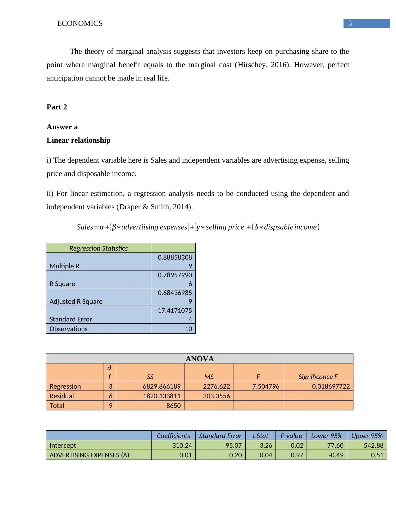
i) The dependent variable here is Sales and independent variables are advertising expense, selling
price and disposable income.
ii) For linear estimation, a regression analysis needs to be conducted using the dependent and
independent variables (Draper & Smith, 2014).
Sales=α + ( β∗advertiising expenses ) + ( γ∗selling price ) +(δ∗dispsable income)
Regression Statistics
Multiple R
0.88858308
9
R Square
0.78957990
6
Adjusted R Square
0.68436985
9
Standard Error
17.4171075
4
Observations 10
ANOVA
d
f SS MS F Significance F
Regression 3 6829.866189 2276.622 7.504796 0.018697722
Residual 6 1820.133811 303.3556
Total 9 8650
Coefficients Standard Error t Stat P-value Lower 95% Upper 95%
Intercept 310.24 95.07 3.26 0.02 77.60 542.88
ADVERTISING EXPENSES (A) 0.01 0.20 0.04 0.97 -0.49 0.51
The theory of marginal analysis suggests that investors keep on purchasing share to the
point where marginal benefit equals to the marginal cost (Hirschey, 2016). However, perfect
anticipation cannot be made in real life.
Part 2
Answer a
Linear relationship
i) The dependent variable here is Sales and independent variables are advertising expense, selling
price and disposable income.
ii) For linear estimation, a regression analysis needs to be conducted using the dependent and
independent variables (Draper & Smith, 2014).
Sales=α + ( β∗advertiising expenses ) + ( γ∗selling price ) +(δ∗dispsable income)
Regression Statistics
Multiple R
0.88858308
9
R Square
0.78957990
6
Adjusted R Square
0.68436985
9
Standard Error
17.4171075
4
Observations 10
ANOVA
d
f SS MS F Significance F
Regression 3 6829.866189 2276.622 7.504796 0.018697722
Residual 6 1820.133811 303.3556
Total 9 8650
Coefficients Standard Error t Stat P-value Lower 95% Upper 95%
Intercept 310.24 95.07 3.26 0.02 77.60 542.88
ADVERTISING EXPENSES (A) 0.01 0.20 0.04 0.97 -0.49 0.51
⊘ This is a preview!⊘
Do you want full access?
Subscribe today to unlock all pages.
Trusted by 1+ million students worldwide
6ECONOMICS
($'000)
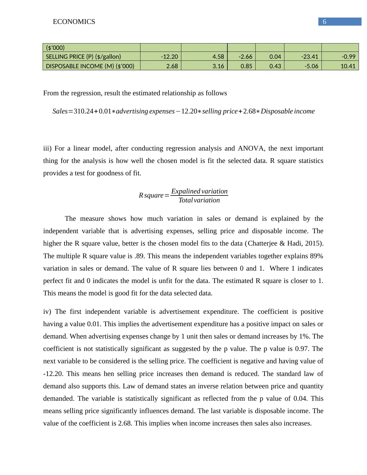
SELLING PRICE (P) ($/gallon) -12.20 4.58 -2.66 0.04 -23.41 -0.99
DISPOSABLE INCOME (M) ($'000) 2.68 3.16 0.85 0.43 -5.06 10.41
From the regression, result the estimated relationship as follows
Sales=310.24+0.01∗advertising expenses−12.20∗selling price+ 2.68∗Disposable income
iii) For a linear model, after conducting regression analysis and ANOVA, the next important
thing for the analysis is how well the chosen model is fit the selected data. R square statistics
provides a test for goodness of fit.
R square= Expalined variation
Total variation
The measure shows how much variation in sales or demand is explained by the
independent variable that is advertising expenses, selling price and disposable income. The
higher the R square value, better is the chosen model fits to the data (Chatterjee & Hadi, 2015).
The multiple R square value is .89. This means the independent variables together explains 89%
variation in sales or demand. The value of R square lies between 0 and 1. Where 1 indicates
perfect fit and 0 indicates the model is unfit for the data. The estimated R square is closer to 1.
This means the model is good fit for the data selected data.
iv) The first independent variable is advertisement expenditure. The coefficient is positive
having a value 0.01. This implies the advertisement expenditure has a positive impact on sales or
demand. When advertising expenses change by 1 unit then sales or demand increases by 1%. The
coefficient is not statistically significant as suggested by the p value. The p value is 0.97. The
next variable to be considered is the selling price. The coefficient is negative and having value of
-12.20. This means hen selling price increases then demand is reduced. The standard law of
demand also supports this. Law of demand states an inverse relation between price and quantity
demanded. The variable is statistically significant as reflected from the p value of 0.04. This
means selling price significantly influences demand. The last variable is disposable income. The
value of the coefficient is 2.68. This implies when income increases then sales also increases.
($'000)
SELLING PRICE (P) ($/gallon) -12.20 4.58 -2.66 0.04 -23.41 -0.99
DISPOSABLE INCOME (M) ($'000) 2.68 3.16 0.85 0.43 -5.06 10.41
From the regression, result the estimated relationship as follows
Sales=310.24+0.01∗advertising expenses−12.20∗selling price+ 2.68∗Disposable income
iii) For a linear model, after conducting regression analysis and ANOVA, the next important
thing for the analysis is how well the chosen model is fit the selected data. R square statistics
provides a test for goodness of fit.
R square= Expalined variation
Total variation
The measure shows how much variation in sales or demand is explained by the
independent variable that is advertising expenses, selling price and disposable income. The
higher the R square value, better is the chosen model fits to the data (Chatterjee & Hadi, 2015).
The multiple R square value is .89. This means the independent variables together explains 89%
variation in sales or demand. The value of R square lies between 0 and 1. Where 1 indicates
perfect fit and 0 indicates the model is unfit for the data. The estimated R square is closer to 1.
This means the model is good fit for the data selected data.
iv) The first independent variable is advertisement expenditure. The coefficient is positive
having a value 0.01. This implies the advertisement expenditure has a positive impact on sales or
demand. When advertising expenses change by 1 unit then sales or demand increases by 1%. The
coefficient is not statistically significant as suggested by the p value. The p value is 0.97. The
next variable to be considered is the selling price. The coefficient is negative and having value of
-12.20. This means hen selling price increases then demand is reduced. The standard law of
demand also supports this. Law of demand states an inverse relation between price and quantity
demanded. The variable is statistically significant as reflected from the p value of 0.04. This
means selling price significantly influences demand. The last variable is disposable income. The
value of the coefficient is 2.68. This implies when income increases then sales also increases.
Paraphrase This Document
Need a fresh take? Get an instant paraphrase of this document with our AI Paraphraser
7ECONOMICS
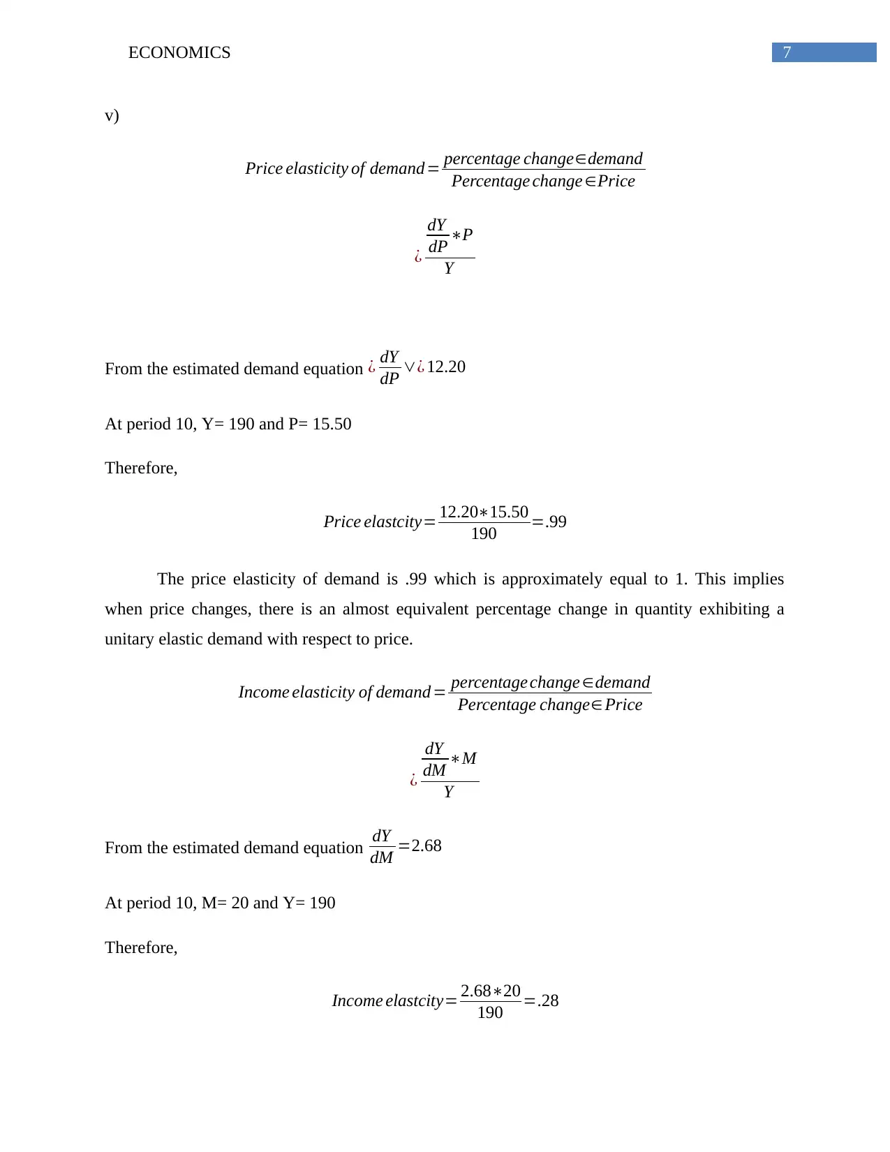
v)
Price elasticity of demand= percentage change∈demand
Percentage change ∈Price
¿
dY
dP ∗P
Y
From the estimated demand equation ¿ dY
dP ∨¿ 12.20
At period 10, Y= 190 and P= 15.50
Therefore,
Price elastcity= 12.20∗15.50
190 =.99
The price elasticity of demand is .99 which is approximately equal to 1. This implies
when price changes, there is an almost equivalent percentage change in quantity exhibiting a
unitary elastic demand with respect to price.
Income elasticity of demand = percentage change ∈demand
Percentage change∈Price
¿
dY
dM ∗M
Y
From the estimated demand equation dY
dM =2.68
At period 10, M= 20 and Y= 190
Therefore,
Income elastcity= 2.68∗20
190 =.28
8ECONOMICS
Income elasticity of demand is less than 1. This means proportionate change in demand is
less than the proportionate change in income making demand relatively inelastic with respect to
income.
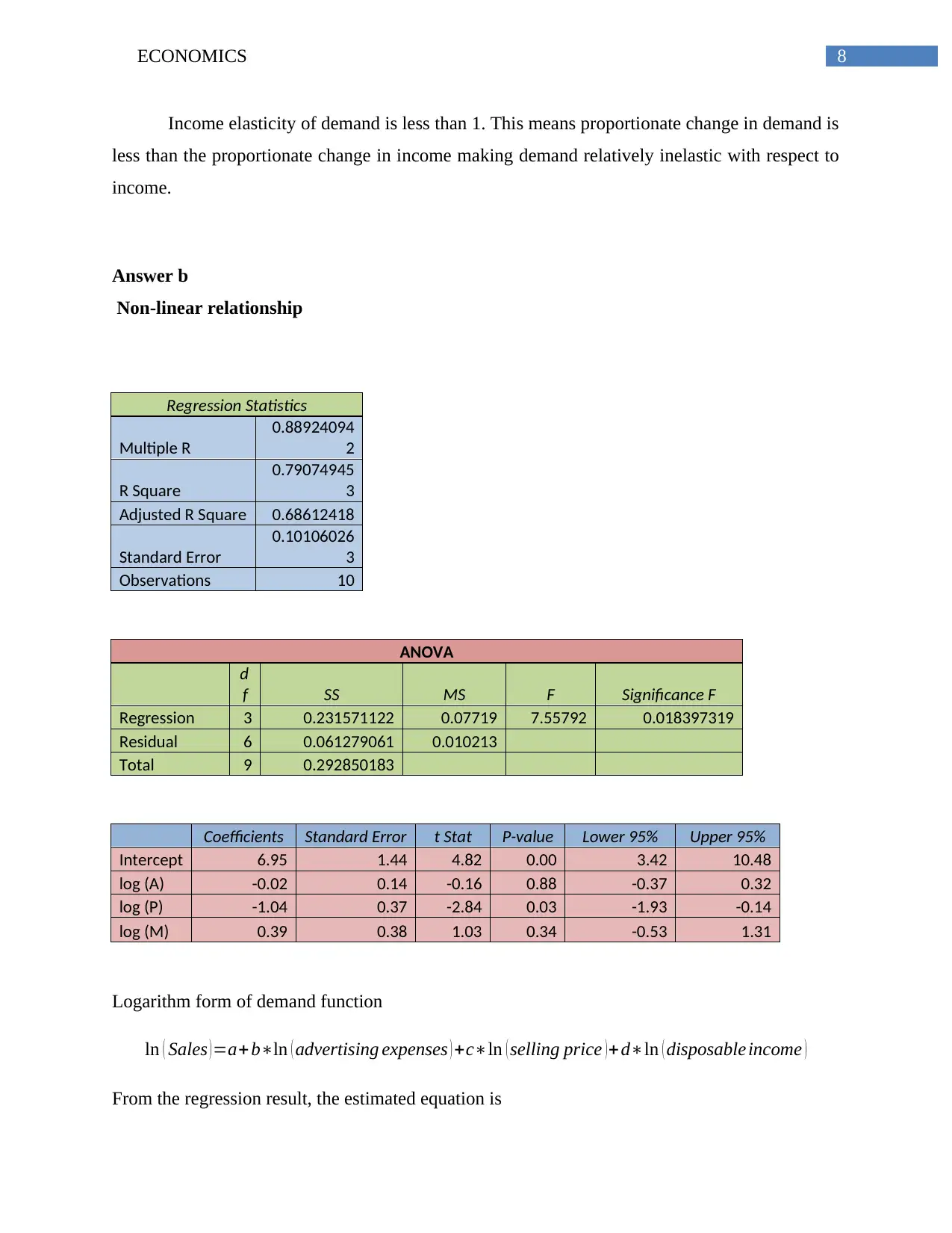
Answer b
Non-linear relationship
Regression Statistics
Multiple R
0.88924094
2
R Square
0.79074945
3
Adjusted R Square 0.68612418
Standard Error
0.10106026
3
Observations 10
ANOVA
d
f SS MS F Significance F
Regression 3 0.231571122 0.07719 7.55792 0.018397319
Residual 6 0.061279061 0.010213
Total 9 0.292850183
Coefficients Standard Error t Stat P-value Lower 95% Upper 95%
Intercept 6.95 1.44 4.82 0.00 3.42 10.48
log (A) -0.02 0.14 -0.16 0.88 -0.37 0.32
log (P) -1.04 0.37 -2.84 0.03 -1.93 -0.14
log (M) 0.39 0.38 1.03 0.34 -0.53 1.31
Logarithm form of demand function
ln ( Sales )=a+ b∗ln ( advertising expenses ) +c∗ln ( selling price )+d∗ln ( disposable income )
From the regression result, the estimated equation is
Income elasticity of demand is less than 1. This means proportionate change in demand is
less than the proportionate change in income making demand relatively inelastic with respect to
income.
Answer b
Non-linear relationship
Regression Statistics
Multiple R
0.88924094
2
R Square
0.79074945
3
Adjusted R Square 0.68612418
Standard Error
0.10106026
3
Observations 10
ANOVA
d
f SS MS F Significance F
Regression 3 0.231571122 0.07719 7.55792 0.018397319
Residual 6 0.061279061 0.010213
Total 9 0.292850183
Coefficients Standard Error t Stat P-value Lower 95% Upper 95%
Intercept 6.95 1.44 4.82 0.00 3.42 10.48
log (A) -0.02 0.14 -0.16 0.88 -0.37 0.32
log (P) -1.04 0.37 -2.84 0.03 -1.93 -0.14
log (M) 0.39 0.38 1.03 0.34 -0.53 1.31
Logarithm form of demand function
ln ( Sales )=a+ b∗ln ( advertising expenses ) +c∗ln ( selling price )+d∗ln ( disposable income )
From the regression result, the estimated equation is
⊘ This is a preview!⊘
Do you want full access?
Subscribe today to unlock all pages.
Trusted by 1+ million students worldwide
9ECONOMICS
ln ( Sales ) =6.95−0.02∗log ( A ) −1.04∗log ( P ) +0.39∗log ( M )
ii)The goodness of fitted model is analyzed in terms of obtained R squared value (Cohen et al.,
2013). The R square value is same as obtained for the linear demand function. The estimated
value of multiple R square .89. This means advertising expenses, selling price disposable income
together able to explain 89% variation in demand. This means the logarithm model is also a good
fit.
iii) The coefficient of advertising expenses is -0.02. This implies a negative relation between
sales and expenditure. An increase in advertisement spending likely to decreases the demand.
This is in contrast to the result obtained under for linear demand estimate. In the linear estimate
the coefficient corresponds to advertising spending appears as positive. However, in neither of
the demand function advertise expenditure is statistically significant (Frost, 2013). The
coefficient for sales is -1.04. This means when selling price in increases then sales fall for the
obvious reason. The variable is also statistically significant as like linear demand function.
Therefore, the conclusion about selling price is unambiguous. As far as the disposable income is
concerned, the coefficient is 0.39. That means a rise is income raises demand as well. The
variable again is statistically insignificant same as the linear demand estimate.
Part 3
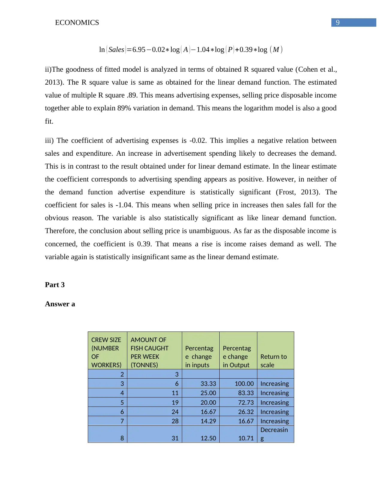
Answer a
CREW SIZE
(NUMBER
OF
WORKERS)
AMOUNT OF
FISH CAUGHT
PER WEEK
(TONNES)
Percentag
e change
in inputs
Percentag
e change
in Output
Return to
scale
2 3
3 6 33.33 100.00 Increasing
4 11 25.00 83.33 Increasing
5 19 20.00 72.73 Increasing
6 24 16.67 26.32 Increasing
7 28 14.29 16.67 Increasing
8 31 12.50 10.71
Decreasin
g
ln ( Sales ) =6.95−0.02∗log ( A ) −1.04∗log ( P ) +0.39∗log ( M )
ii)The goodness of fitted model is analyzed in terms of obtained R squared value (Cohen et al.,
2013). The R square value is same as obtained for the linear demand function. The estimated
value of multiple R square .89. This means advertising expenses, selling price disposable income
together able to explain 89% variation in demand. This means the logarithm model is also a good
fit.
iii) The coefficient of advertising expenses is -0.02. This implies a negative relation between
sales and expenditure. An increase in advertisement spending likely to decreases the demand.
This is in contrast to the result obtained under for linear demand estimate. In the linear estimate
the coefficient corresponds to advertising spending appears as positive. However, in neither of
the demand function advertise expenditure is statistically significant (Frost, 2013). The
coefficient for sales is -1.04. This means when selling price in increases then sales fall for the
obvious reason. The variable is also statistically significant as like linear demand function.
Therefore, the conclusion about selling price is unambiguous. As far as the disposable income is
concerned, the coefficient is 0.39. That means a rise is income raises demand as well. The
variable again is statistically insignificant same as the linear demand estimate.
Part 3
Answer a
CREW SIZE
(NUMBER
OF
WORKERS)
AMOUNT OF
FISH CAUGHT
PER WEEK
(TONNES)
Percentag
e change
in inputs
Percentag
e change
in Output
Return to
scale
2 3
3 6 33.33 100.00 Increasing
4 11 25.00 83.33 Increasing
5 19 20.00 72.73 Increasing
6 24 16.67 26.32 Increasing
7 28 14.29 16.67 Increasing
8 31 12.50 10.71
Decreasin
g
Paraphrase This Document
Need a fresh take? Get an instant paraphrase of this document with our AI Paraphraser
10ECONOMICS
9 33 11.11 6.45
Decreasin
g
10 34 10.00 3.03
Decreasin
g
11 34 9.09 0.00
Decreasin
g
12 33 -100.00 -2.94 Negative
Return to scale shows the relation between inputs and output. If the proportionate change
in output is greater than the proportionate change in inputs then production function said to have
increasing return to scale. If proportionate change in output is less than the proportionate change
in input, then the production function exhibits decreasing return to scale (Baumol & Blinder,
2015). The scale or return is constant in cases where output changes exactly matches with
proportionate change in inputs.
i)
For number of workers ranging from 3 to7, there are increasing return to scale. Within this range
the percentage change in total amount of fish caught exceeds the percentage change in number of
workers.
For number of workers ranging from 8 to 11, there are decreasing return to scale. Here,
percentage change in number of workers is greater than the amount of fish caught that is the total
output.
There is no level of production having constant return to scale.
When number of workers is 12 there are negative returns. At this level when number of worker
increases then total amount of fish caught decreases, hence exhibiting negative returns.
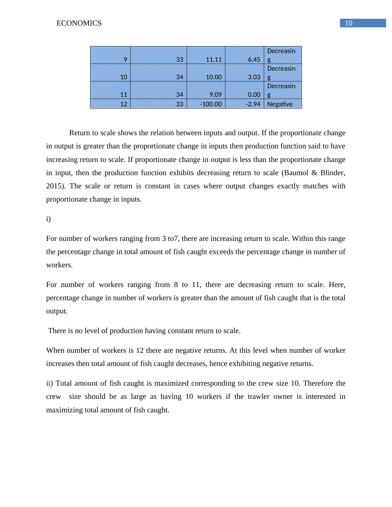
ii) Total amount of fish caught is maximized corresponding to the crew size 10. Therefore the
crew size should be as large as having 10 workers if the trawler owner is interested in
maximizing total amount of fish caught.
9 33 11.11 6.45
Decreasin
g
10 34 10.00 3.03
Decreasin
g
11 34 9.09 0.00
Decreasin
g
12 33 -100.00 -2.94 Negative
Return to scale shows the relation between inputs and output. If the proportionate change
in output is greater than the proportionate change in inputs then production function said to have
increasing return to scale. If proportionate change in output is less than the proportionate change
in input, then the production function exhibits decreasing return to scale (Baumol & Blinder,
2015). The scale or return is constant in cases where output changes exactly matches with
proportionate change in inputs.
i)
For number of workers ranging from 3 to7, there are increasing return to scale. Within this range
the percentage change in total amount of fish caught exceeds the percentage change in number of
workers.
For number of workers ranging from 8 to 11, there are decreasing return to scale. Here,
percentage change in number of workers is greater than the amount of fish caught that is the total
output.
There is no level of production having constant return to scale.
When number of workers is 12 there are negative returns. At this level when number of worker
increases then total amount of fish caught decreases, hence exhibiting negative returns.
ii) Total amount of fish caught is maximized corresponding to the crew size 10. Therefore the
crew size should be as large as having 10 workers if the trawler owner is interested in
maximizing total amount of fish caught.
11ECONOMICS
0 2 4 6 8 10 12 14
0
5
10
15
20
25
30
35
40
Total Amount of Fish caught per week (Tonnes)
TOTAL AMOUNT
OF FISH CAUGHT
PER WEEK
(TONNES)
Number of workers
Total amout of fish caught
Figure 1: Total amount of fish caught corresponding to the crew size
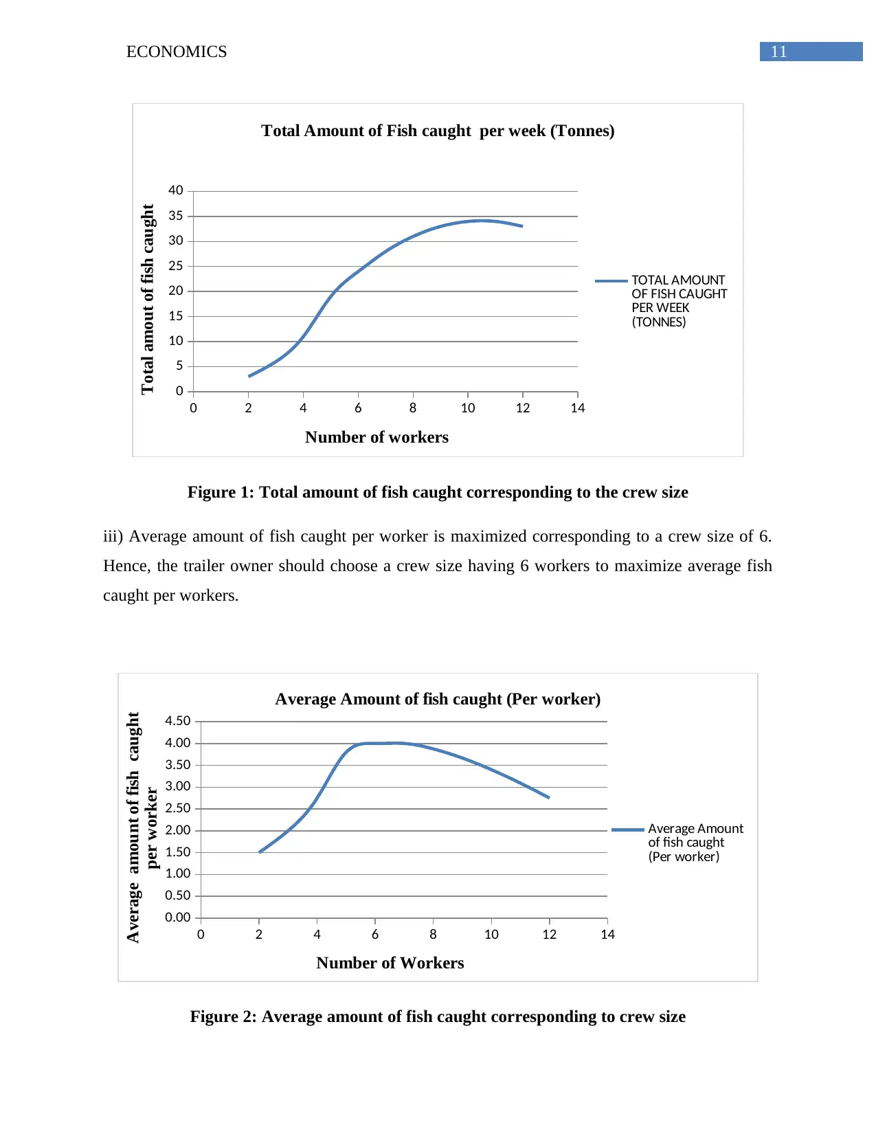
iii) Average amount of fish caught per worker is maximized corresponding to a crew size of 6.
Hence, the trailer owner should choose a crew size having 6 workers to maximize average fish
caught per workers.
0 2 4 6 8 10 12 14
0.00
0.50
1.00
1.50
2.00
2.50
3.00
3.50
4.00
4.50
Average Amount of fish caught (Per worker)
Average Amount
of fish caught
(Per worker)
Number of Workers
Average amount of fish caught
per worker
Figure 2: Average amount of fish caught corresponding to crew size
0 2 4 6 8 10 12 14
0
5
10
15
20
25
30
35
40
Total Amount of Fish caught per week (Tonnes)
TOTAL AMOUNT
OF FISH CAUGHT
PER WEEK
(TONNES)
Number of workers
Total amout of fish caught
Figure 1: Total amount of fish caught corresponding to the crew size
iii) Average amount of fish caught per worker is maximized corresponding to a crew size of 6.
Hence, the trailer owner should choose a crew size having 6 workers to maximize average fish
caught per workers.
0 2 4 6 8 10 12 14
0.00
0.50
1.00
1.50
2.00
2.50
3.00
3.50
4.00
4.50
Average Amount of fish caught (Per worker)
Average Amount
of fish caught
(Per worker)
Number of Workers
Average amount of fish caught
per worker
Figure 2: Average amount of fish caught corresponding to crew size
⊘ This is a preview!⊘
Do you want full access?
Subscribe today to unlock all pages.
Trusted by 1+ million students worldwide
1 out of 23
Related Documents


Your All-in-One AI-Powered Toolkit for Academic Success.
+13062052269
info@desklib.com
Available 24*7 on WhatsApp / Email
![[object Object]](/_next/static/media/star-bottom.7253800d.svg)
Unlock your academic potential
Copyright © 2020–2026 A2Z Services. All Rights Reserved. Developed and managed by ZUCOL.