University Economics Assignment: Consumer Behavior and Analysis

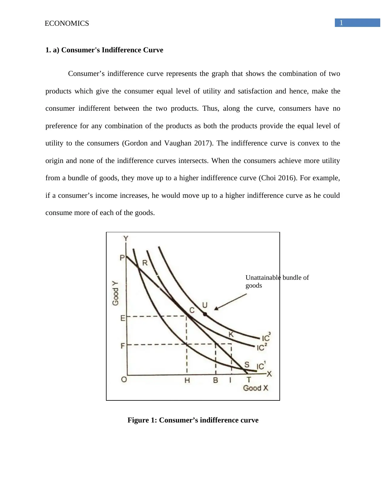
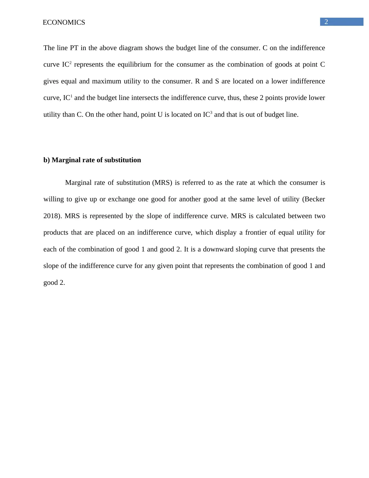
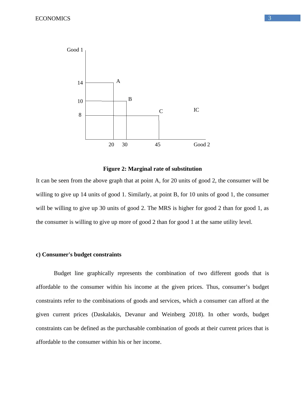
This economics assignment explores key concepts in consumer behavior. It begins by defining and illustrating the consumer's indifference curve, explaining how it represents combinations of goods providing equal utility. The assignment then delves into the marginal rate of substitution (MRS), demonstrating how consumers trade one good for another while maintaining utility. Consumer budget constraints, which limit consumption based on income and prices, are also explained. The law of diminishing marginal utility is discussed, highlighting how the satisfaction from consuming additional units of a good decreases. The assignment then examines income and substitution effects, which explain how changes in price affect consumer demand. Finally, the assignment analyzes behavioral economics and the reasons behind irrational consumer behavior, including cognitive biases, herding, and other psychological factors that deviate from rational choice theory, providing a comprehensive overview of consumer decision-making processes.

Running head: ECONOMICS
Economics
Name of the Student:
Name of the University:
Author note:

1ECONOMICS
1. a) Consumer's Indifference Curve
Consumer’s indifference curve represents the graph that shows the combination of two
products which give the consumer equal level of utility and satisfaction and hence, make the
consumer indifferent between the two products. Thus, along the curve, consumers have no
preference for any combination of the products as both the products provide the equal level of
utility to the consumers (Gordon and Vaughan 2017). The indifference curve is convex to the
origin and none of the indifference curves intersects. When the consumers achieve more utility
from a bundle of goods, they move up to a higher indifference curve (Choi 2016). For example,
if a consumer’s income increases, he would move up to a higher indifference curve as he could
consume more of each of the goods.
Figure 1: Consumer’s indifference curve
Unattainable bundle of
goods

2ECONOMICS
The line PT in the above diagram shows the budget line of the consumer. C on the indifference
curve IC2 represents the equilibrium for the consumer as the combination of goods at point C
gives equal and maximum utility to the consumer. R and S are located on a lower indifference
curve, IC1 and the budget line intersects the indifference curve, thus, these 2 points provide lower
utility than C. On the other hand, point U is located on IC3 and that is out of budget line.
b) Marginal rate of substitution
Marginal rate of substitution (MRS) is referred to as the rate at which the consumer is
willing to give up or exchange one good for another good at the same level of utility (Becker
2018). MRS is represented by the slope of indifference curve. MRS is calculated between two
products that are placed on an indifference curve, which display a frontier of equal utility for
each of the combination of good 1 and good 2. It is a downward sloping curve that presents the
slope of the indifference curve for any given point that represents the combination of good 1 and
good 2.

3ECONOMICS
Good 1
Good 2
IC
8
10
14 A
B
C
20 30 45
Figure 2: Marginal rate of substitution
It can be seen from the above graph that at point A, for 20 units of good 2, the consumer will be
willing to give up 14 units of good 1. Similarly, at point B, for 10 units of good 1, the consumer
will be willing to give up 30 units of good 2. The MRS is higher for good 2 than for good 1, as
the consumer is willing to give up more of good 2 than for good 1 at the same utility level.
c) Consumer's budget constraints
Budget line graphically represents the combination of two different goods that is
affordable to the consumer within his income at the given prices. Thus, consumer’s budget
constraints refer to the combinations of goods and services, which a consumer can afford at the
given current prices (Daskalakis, Devanur and Weinberg 2018). In other words, budget
constraints can be defined as the purchasable combination of goods at their current prices that is
affordable to the consumer within his or her income.

4ECONOMICS
Thus, if M is the consumer’s income for purchasing good X and good Y and PX and PY
are the respective prices, then the budget line is defined as:
PX * X + PY * Y = M
And the budget constraint can be defined as:
PX * X + PY * Y <= M
Figure 3: Consumer's budget line and budget constraint
Any combination of good X and good Y that is below the budget line AB shown in the above
diagram, such as, C, is attainable and it is a budget constraint. However, any combination of X
and Y, which is above the budget line, such as, at point D, is unattainable, as it goes beyond the
purchasing power of the consumer.
d) Diminishing marginal utility
The law of diminishing marginal utility says that with increasing consumption of a
commodity, the utility derived decreases with every successive units of the commodity while

5ECONOMICS
other things remaining same. As stated by Kauder (2015), marginal utility is derived from the
change in utility derived from consumption of each additional unit of a commodity, and as per
the law of diminishing marginal utility, the marginal utility from the consumption of each
additional unit of a commodity diminishes provided other things remaining same. Although the
total utility from the consumption increases, the marginal utility decreases as per the law of
diminishing marginal utility (Tan and Zhang 2015).
For example, a consumer consumes 6 units of good X. The first unit gives him 20 utils
(units to measure utility) and with the consumption of the 2nd unit, the utils decreased to 15 and
with 3rd unit, the consumer derives 10 utils. Thus, the marginal utility is diminishing with each
unit of consumption of good X, while the total utility is increasing.
Consumption unit of good X Marginal utility Total utility
1 20 20
2 15 35
3 10 45
4 5 50
5 0 50
6 -5 45
Table 1: Diminishing marginal utility
Thus, at one point, the marginal utility becomes 0 and afterwards it becomes negative. At that
point, the total utility starts to decrease as seen in the table above.

6ECONOMICS
e) Income and substitution effects
When the price of a commodity increases, there are two types of effects, income and
substitution effects. Income effect refers to the impact of change in the real income of the
consumer due to change in the price of a commodity. As highlighted by Berry et al. (2018), when
the price of a commodity increases, it reduces the real or disposable income of the consumer and
the fall in real income results in reduced demand for the commodity. For example, if the price of
apples increases, then higher price would discourage consumers to purchase fewer amount of
apples as higher price affects the disposable income of the consumers and thus, demand for
apples falls. It is known as income effect.
On the other hand, substitution effect refers to the impact of change in the relative income
and prices of the commodity on the consumption pattern of the consumer. As stated by
Hayakawa and Venieris (2016), substitution effect represents that increased price of a
commodity encourages the consumer to purchase alternative or substitute commodity. In other
words, substitution effect influences the consumer to buy different commodities due to price rise
of one commodity with income level remaining the same. For example, if the price of
commodity X increases, with income level remaining same, the consumer might change his
preference and purchase a substitute commodity instead of X. This is called substitution effect.
2) 'Behavioral Economics' and critically evaluation of the reasons behind irrational
behaviors of consumers
Behavioral Economics represents the psychological study of the individuals and
institutions in the context of the process of economic decision making. As pointed out by

7ECONOMICS
Wilkinson and Klaes (2017), behavioral economics is the branch of study that deals with the
psychological, emotional, cognitive, social and cultural factors that affect the economic decisions
of the individuals and organizations and their difference from the classical theory.
Rational behavior of the consumers is studied in behavioral economics. Economic
decisions of the consumers are based on various aspects and those are subject to constraints. As
consumers aim to maximize their welfare and utility within the constraints of limited income by
choosing the appropriate bundle of goods, the incomplete information often causes welfare loss
of both the consumers and producers (Oliveira-Castro, Cavalcanti and Foxall 2015). Thus,
according to the rational choice theory, consumers take rational economic decision by weighing
the cost and benefit of each option.
Irrational behavior can be of the following types, such as, irrational exuberance, herding,
cognitive bias, demerit bias, status quo bias, discrimination, sunk cost fallacy, and lack of control
(Thaler 2017). Thus, it can be stated that irritation behavior arises when the consumers believe in
over optimism, especially in case of asset bubble. When the price of shares rises, people have a
tendency to keep on buying more. In case of herding, individuals assume that majority of the
peers are correct and they tend follow the economic decision made by the masses (Cartwright
2018). Under cognitive bias, people are unaware of the irrational decision made by them and
these choices are made under the influence of emotions or impulses. Under status quo, people
stick to the default option even if it is not the best option rather than spending time to find the
best alternative. In case of demerit goods, such as, drugs, tobacco or alcohol, addiction plays a
major role in influencing the irrational consumption decision. Addiction also results in lack of
control and irrational behavior can be seen in case of consumption of harmful goods (MacKillop
2016). Discrimination often occurs in the labor market where irrational behavior is displayed

8ECONOMICS
based on biasness (Albanese 2015). Sunk cost fallacy is displayed when individuals cannot part
ways with their unproductive resources due to emotional attachment. Thus, various emotional,
cultural, social factors lead to irrational behavior of consumers, which leads to economic
situations like market failure, financial instability and higher profit by organizations through
price discrimination (Kanev and Terziev 2017).

9ECONOMICS
References
Albanese, P., 2015. Inside economic man: behavioral economics and consumer behavior.
In Handbook of contemporary behavioral economics (pp. 25-45). Routledge.
Becker, G., 2015. Marginal Rate of Substitution. Wiley Encyclopedia of Management, pp.1-1.
Berry, K., Bayham, J., Meyer, S.R. and Fenichel, E.P., 2018. The allocation of time and risk of
Lyme: a case of ecosystem service income and substitution effects. Environmental and resource
economics, 70(3), pp.631-650.
Cartwright, E., 2018. Behavioral economics. Routledge.
Choi, H., 2016. Grossman-Helpman's Singular Indifference Curve. Available at SSRN 2783248.
Daskalakis, C., Devanur, N.R. and Weinberg, S.M., 2018. Revenue maximization and ex-post
budget constraints. ACM Transactions on Economics and Computation (TEAC), 6(3-4), p.20.
Gordon, D. and Vaughan, R., 2017. Thick Indifference Curves, Marketing and Behavioral
Economics. Journal of Progressive Research in Social Sciences, 6(1), pp.422-425.
Hayakawa, H. and Venieris, Y., 2016. Consumer interdependence via reference groups.
In Behavioral Interactions, Markets, and Economic Dynamics (pp. 81-99). Springer, Tokyo.
Kanev, D. and Terziev, V., 2017. Behavioral economics: development, condition and
perspectives. IJASOS-International E-Journal of Advances in Social Sciences, 3(8).
Kauder, E., 2015. History of marginal utility theory (Vol. 2238). Princeton University Press.

10ECONOMICS
MacKillop, J., 2016. The behavioral economics and neuroeconomics of alcohol use
disorders. Alcoholism: Clinical and Experimental Research, 40(4), pp.672-685.
Oliveira-Castro, J.M., Cavalcanti, P.R. and Foxall, G.R., 2015. What do consumers
maximize?. The Routledge Companion to Consumer Behavior Analysis, p.202.
Tan, L. and Zhang, Y., 2015. Optimal resource allocation with principle of equality and
diminishing marginal utility in wireless networks. Wireless Personal Communications, 84(1),
pp.671-693.
Thaler, R.H., 2017. Behavioral economics. Journal of Political Economy, 125(6), pp.1799-1805.
Wilkinson, N. and Klaes, M., 2017. An introduction to behavioral economics. Macmillan
International Higher Education.