Consumption Function and Business Cycles in International Economics

This report provides an analysis of international economics, focusing on the consumption function and business cycles. It explains the relationship between disposable income and consumption, illustrating how households begin to save. The report further delves into the phases of business cycles, including expansion, recession, depression, and recovery, and their effects on unemployment and inflation. It also discusses the interplay between Okun's Law and the Phillips Curve, highlighting the inverse relationships between output, unemployment, and inflation rates. The analysis incorporates the impact of economic policies on mitigating economic downturns, making it a comprehensive overview of key concepts in international economics and their practical implications.

Running head: INTERNATIONAL ECONOMICS
International Economics
Name of the Student:
Name of the University:
Author’s Note:

2INTERNATIONAL ECONOMICS
Table of Contents
Answer to Question 1......................................................................................................................3
Part 1a).............................................................................................................................................3
Part 1b).............................................................................................................................................5
Answer to Question 2......................................................................................................................5
Part 2a).............................................................................................................................................6
Part 2b).............................................................................................................................................7
References:......................................................................................................................................9

3INTERNATIONAL ECONOMICS
Answer to Question 1
The consumption function for the given question is given as
C=a+ b∗ ( Disposable Income )
The C here represent consumption, as autonomous consumption and b as MPC as given in the
equation. “a” is considered to be the minimum consumption that need to be incurred if “b” is
MPC (marginal propensity to consume), the slope of consumption curve. MPC is the
proportionate change in consumption as a resultant change in income (Mullbauer 2016). Hence,
as per the first assumption, if disposable income (Yd) is zero, then consumption will still be
positive.
Part 1a)
0 50 100 150 200 250 300 350 400 450
0
50
100
150
200
250
300
350
400
450
Consumption Function
Initial Consumption Curve
New Consumption Curve
Disposable Income (Yd)
Consumption
A
(200,200)
B(335,350)
Figure 1: Consumption Function

4INTERNATIONAL ECONOMICS
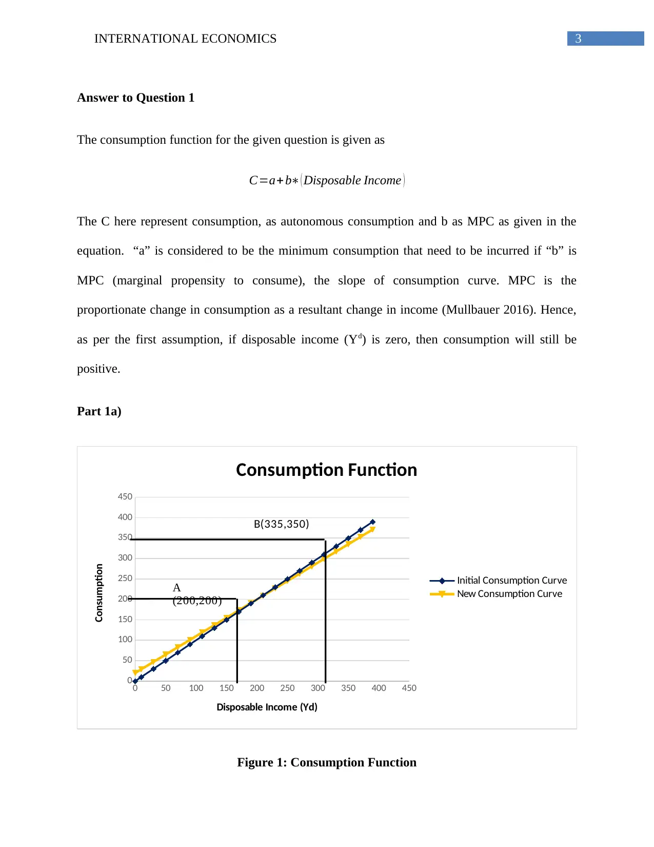
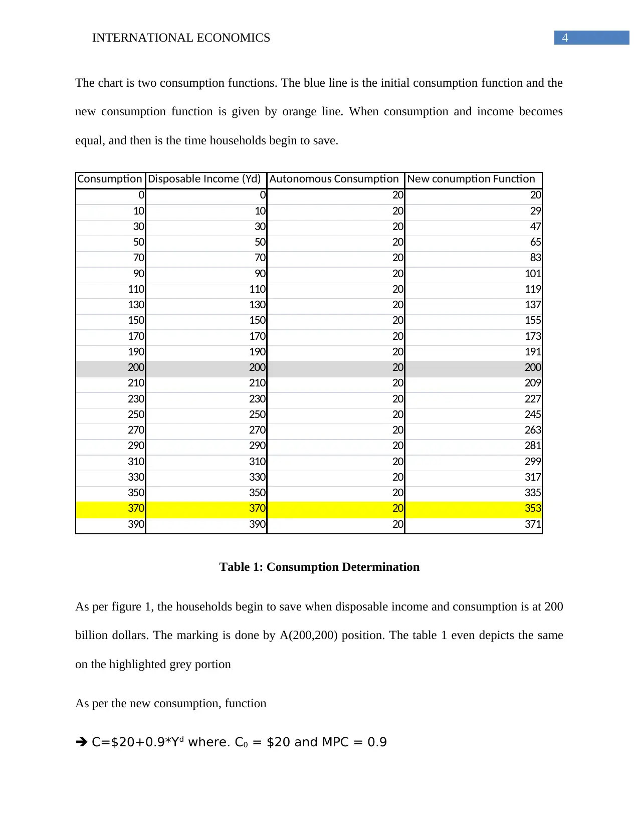
The chart is two consumption functions. The blue line is the initial consumption function and the
new consumption function is given by orange line. When consumption and income becomes
equal, and then is the time households begin to save.
Consumption Disposable Income (Yd) Autonomous Consumption New conumption Function
0 0 20 20
10 10 20 29
30 30 20 47
50 50 20 65
70 70 20 83
90 90 20 101
110 110 20 119
130 130 20 137
150 150 20 155
170 170 20 173
190 190 20 191
200 200 20 200
210 210 20 209
230 230 20 227
250 250 20 245
270 270 20 263
290 290 20 281
310 310 20 299
330 330 20 317
350 350 20 335
370 370 20 353
390 390 20 371
Table 1: Consumption Determination
As per figure 1, the households begin to save when disposable income and consumption is at 200
billion dollars. The marking is done by A(200,200) position. The table 1 even depicts the same
on the highlighted grey portion
As per the new consumption, function
 C=$20+0.9*Yd where. C0 = $20 and MPC = 0.9

5INTERNATIONAL ECONOMICS
C =$20+0.9*Yd = $20+0.9*200 = 20 + 180 = 200 (When Yd = 200 then, C
= 200)
Part 1b)
When income rises by $150 after point A then consumption fill be
 C=$20+0.9*Yd where. C0 = $20 and MPC = 0.9
C =$20+0.9*Yd = $20+0.9*(200+150) = 20 + 0.9*350 = 20+315 = 335
(When Yd = 350 then, C = 335).
As per Figure 1, the same has been indicated in the chart with point B (335,
350)
Answer to Question 2
Economic policy is governed by two central reasons one is growth and other is stabilization in
business cycles. The interest is even influenced by institutions to mitigate the distress in
downturns in the economy through implication of government policies whether monetary or
fiscal in nature (Bhattarai, Lee and Park 2016). Business cycles and economic growth are closely
related to each other because the fluctuation is business cycles are measured by the real GDP.
However, the GDP do not remain stagnant and leas to continuous changes due to many economic
and non-economic reasons.
On the contrary, based on this explanation, it is often implied that log term economic growth is
“real” in nature and is often affected by productivity in physical and human resources. In relation
to this, business cycle theories not only disagree with the comparative roles of monetary and real

6INTERNATIONAL ECONOMICS
factors but even states that short terms fluctuations does not affect the secular growth (Galí
2015).
Part 2a)
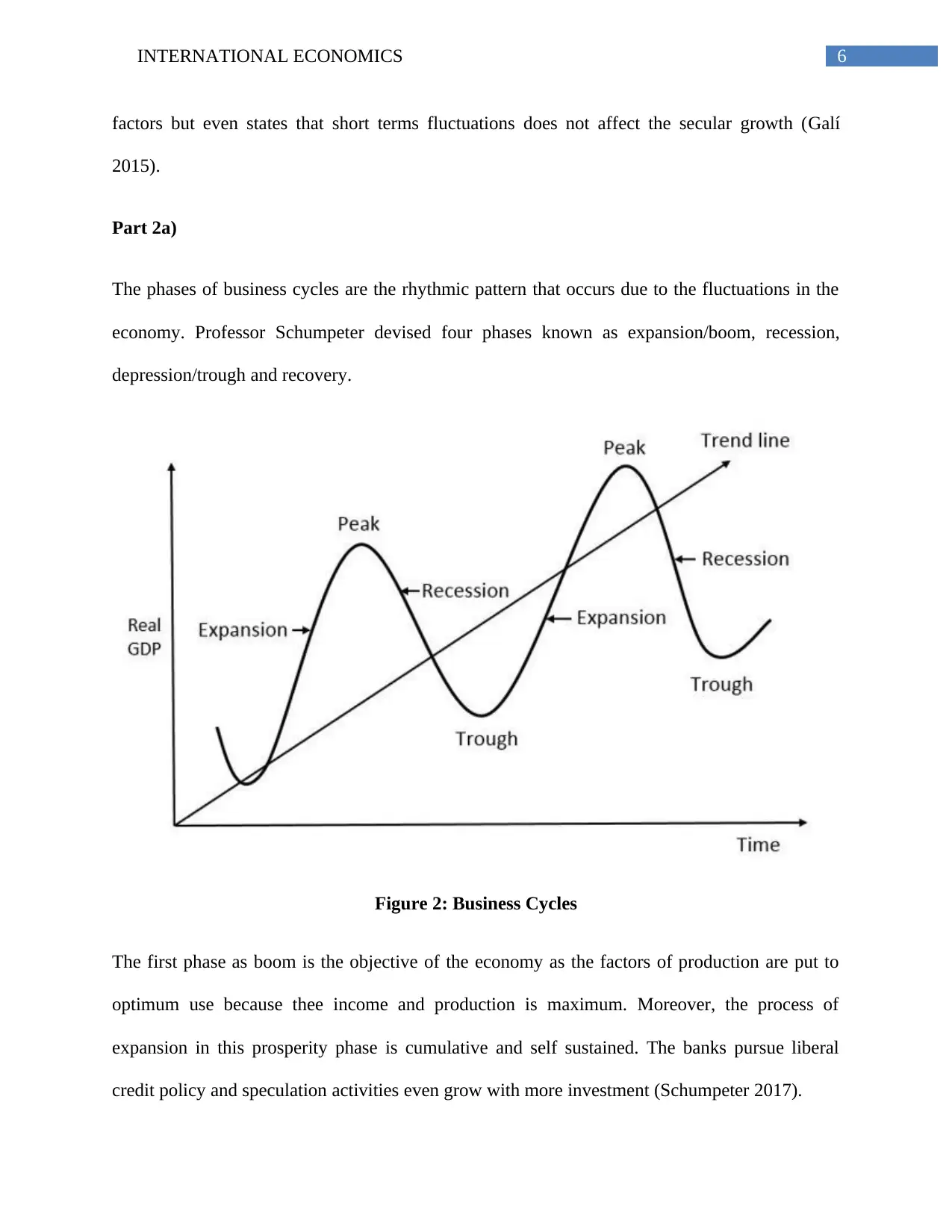
The phases of business cycles are the rhythmic pattern that occurs due to the fluctuations in the
economy. Professor Schumpeter devised four phases known as expansion/boom, recession,
depression/trough and recovery.
Figure 2: Business Cycles
The first phase as boom is the objective of the economy as the factors of production are put to
optimum use because thee income and production is maximum. Moreover, the process of
expansion in this prosperity phase is cumulative and self sustained. The banks pursue liberal
credit policy and speculation activities even grow with more investment (Schumpeter 2017).

7INTERNATIONAL ECONOMICS
The second phase, the recession phase in which inflations begins to rise with widespread
contraction of business activity and decline for wages, output, production and trade. The great
recession had been experienced in 1961-62 when the downturn hit the farms badly and breaking
the vicious cycle that sent inflation to an all time high followed by 2008 “the great recession”
where the main issue had been housing bubble, credit concerns and energy pries recording a new
high.
The third phase as depression is the best described phase by 1930’s where level of output and
production went out of gear, there was widespread unemployment, cash reserves in banks pile
up, price of raw materials fell more than the finished goods. The “Great Depression 1930’s” was
accompanied by all those events with crash in stock market; consumer debt was proliferating and
leading to change in currency system to gold standard with fixed exchange rate (Legrand and
Hagemann 2017).
The last phase is the recovery stage, when the growth is struggling to rise with increase in output,
replaced investments lead to demand for capital good, multiplier and accelerator comes to play
and further, bank loans and advances increases (Mirowski 2015). As the recovery intensified, it
aims for full capacity production return.
Part 2b)
Business cycles have a consistent relationship between unemployment and inflation. This further
has been manifested by two relationships that are through Okun’s Law (inverse relationship
between output and unemployment) and Phillip’s cure (inverse relationship between inflation
and unemployment). In the event of business cycle, unemployment rate rises during contractions
and falls in expansionary phases. The advent of unemployment increases is higher than

8INTERNATIONAL ECONOMICS
unemployment rate falls. However, when it comes to inflation, in contractions, inflations rate
falls as output is falling and increases in expansionary phases (Parkin 2016).
When the output starts falling in the recession/ depression phase, there is still an increase in
inflation from the recovery phase which leads to fall in GDP in the contraction phase of the
economy. The same is applied to unemployment because when entering into recession phase, the
low unemployment rate has already caused an increase in production leading to increasing the
real GDP in the economy (Dorman, 2014).
The contraction phase makes the output falls, unemployment rises and further leads to fall in
inflation. The Philips’ curve well defines the menu of tradeoffs because of the stereotype of
lower unemployment rates with a minor increase in inflation (Mohseni and Jouzaryan 2016).
However, Friedman and Phelps argue regarding the empirical relationship as it had no future
bearing which further reacted differently to economic policies.

9INTERNATIONAL ECONOMICS
References:
Bhattarai, S., Lee, J.W. and Park, W.Y., 2016. Policy regimes, policy shifts, and US business
cycles. Review of Economics and Statistics, 98(5), pp.968-983.
Galí, J., 2015. Monetary policy, inflation, and the business cycle: an introduction to the new
Keynesian framework and its applications. Princeton University Press.
Legrand, M.D.P. and Hagemann, H., 2017. Business Cycles, Growth, And Economic Policy:
Schumpeter And The Great Depression. Journal of the History of Economic Thought, 39(1),
pp.19-33.
Mirowski, P.E., 2015. The Birth of the Business Cycle (RLE: Business Cycles) (Vol. 6).
Routledge.
Mohseni, M. and Jouzaryan, F., 2016. Examining the Effects of Inflation and Unemployment on
Economic Growth in Iran (1996-2012). Procedia Economics and Finance, 36, pp.381-389.
Muellbauer, J., 2016. Macroeconomics and Consumption (No. Paper 811). University of Oxford,
Department of Economics.
Parkin, M., 2016. 9 Unemployment and Inflation: Facts. Unemployment in Western Countries,
p.278.
Schumpeter, J.A., 2017. Essays: on entrepreneurs, innovations, business cycles and the evolution
of capitalism. Routledge.