University Economics Assignment: ECO10250, Decision Making, Sem 1
VerifiedAdded on 2022/10/11
|12
|2172
|19
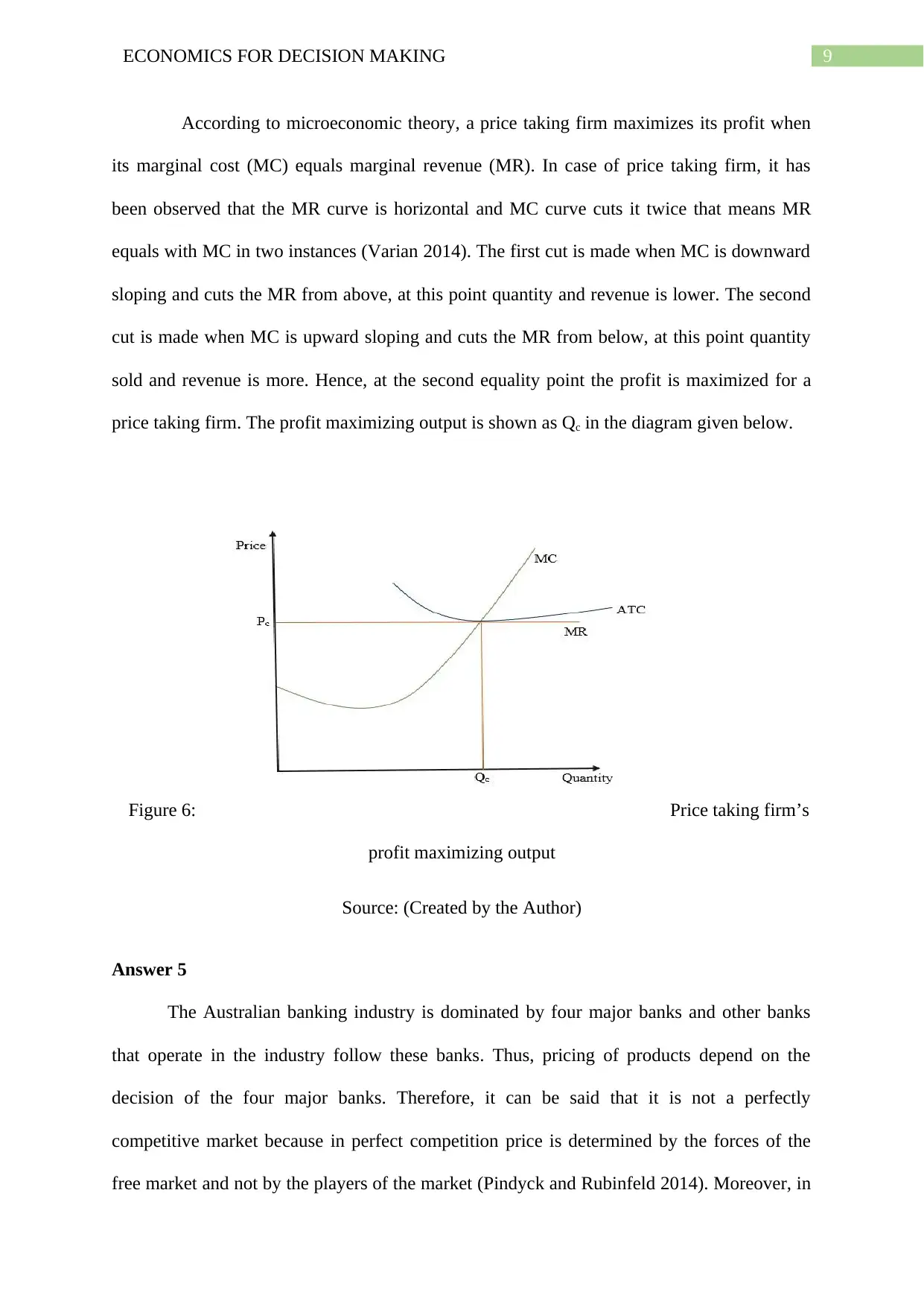
Homework Assignment
AI Summary
This economics assignment solution provides a comprehensive analysis of various economic concepts. It begins with an examination of Joan's production possibility curve, exploring increasing and constant opportunity costs, and efficient and inefficient outcomes. The assignment then delves into supply and demand dynamics, illustrating shifts in curves due to changes in production costs and the impact of government price controls. Elasticity of demand is also explored through calculations and examples of elastic, inelastic, and highly elastic goods, including an analysis of demerit goods. Further, the assignment presents a detailed breakdown of a firm's costs, revenues, and profit maximization in both the short run and long run, including graphical representations. Finally, the assignment concludes with an analysis of the Australian banking industry's market structure, comparing it to perfect competition and monopoly models and discussing its implications for consumers and social welfare.

1 out of 12
Related Documents


Your All-in-One AI-Powered Toolkit for Academic Success.
+13062052269
info@desklib.com
Available 24*7 on WhatsApp / Email
![[object Object]](/_next/static/media/star-bottom.7253800d.svg)
Copyright © 2020–2026 A2Z Services. All Rights Reserved. Developed and managed by ZUCOL.