Economics Assignment - Microeconomics: Elasticity, Market, Monopoly

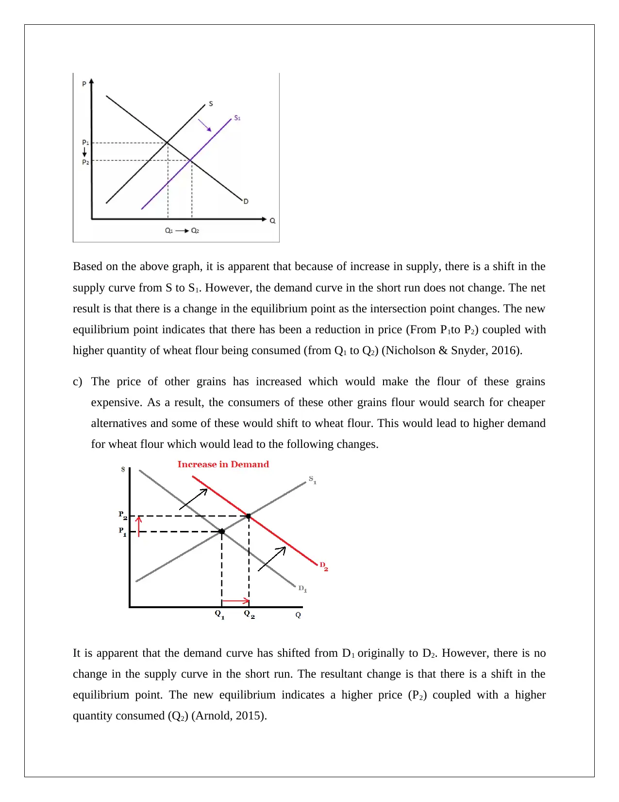
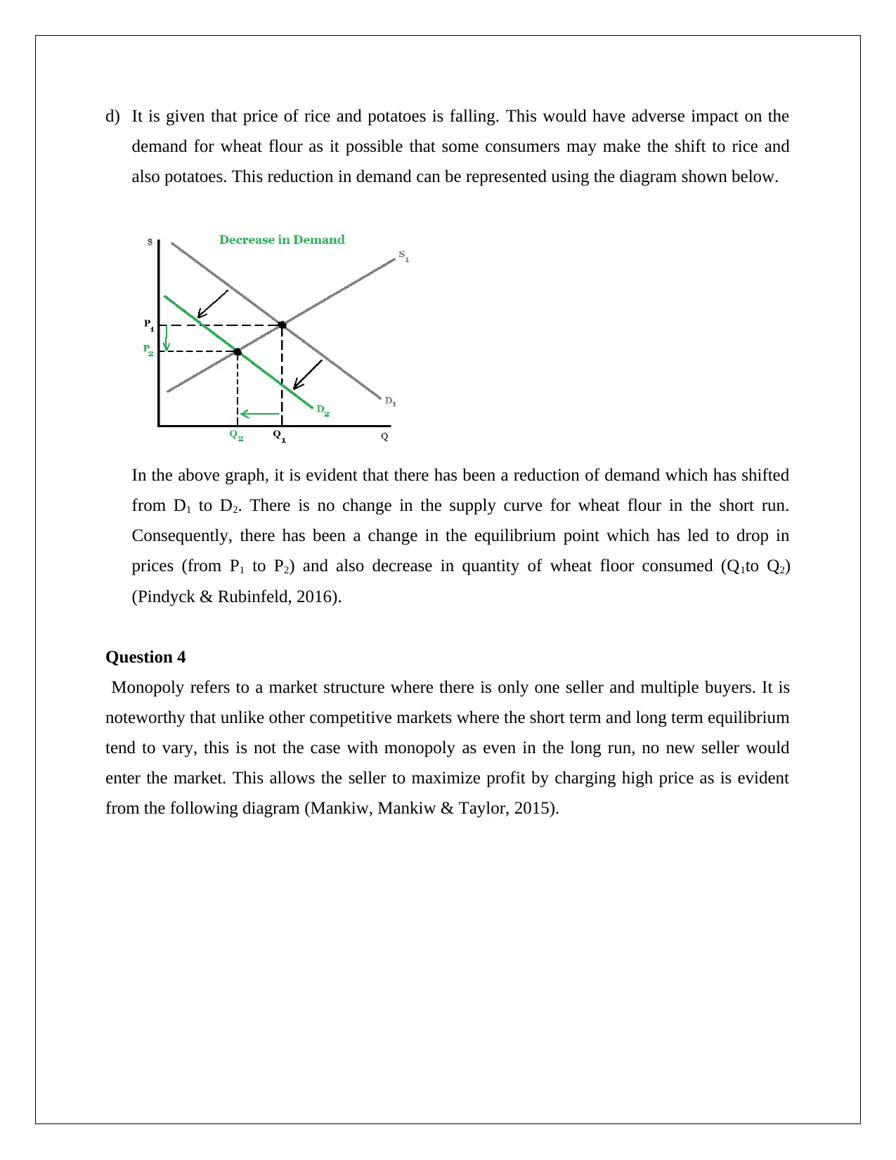
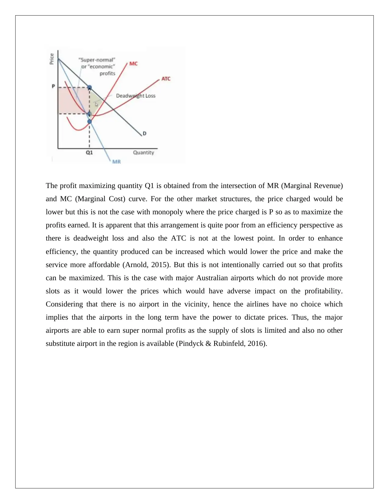
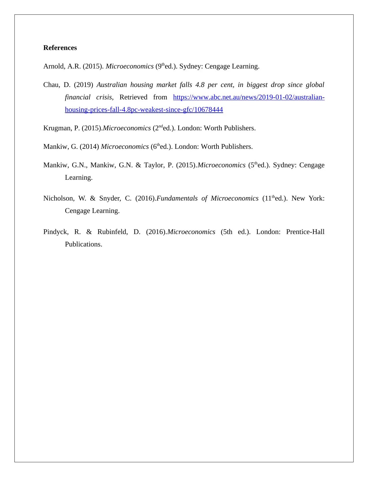
This economics assignment analyzes various microeconomic concepts and real-world market scenarios. It begins by examining the Australian housing market, discussing factors contributing to falling demand and prices, and potential government interventions. The assignment then delves into elasticity, differentiating between price, cross-price, and income elasticities, and analyzing their implications for businesses. Subsequently, it explores supply and demand dynamics, using examples like the wheat flour market to illustrate how shifts in supply and demand curves affect equilibrium price and quantity. Finally, the assignment concludes with a discussion of monopoly market structures, highlighting their characteristics, inefficiencies, and real-world examples such as Australian airports, emphasizing the potential for supernormal profits due to limited competition and supply constraints. The assignment utilizes diagrams to visually represent market changes and includes references to economic literature to support the analysis.

ECONOMICS
STUDENT ID:
[Pick the date]

Question 1
In the recent times, the performance of the Australian housing market has been lackluster. This is
reflective from the fall in house prices in various cities across capital. The extent of fall is clearly
alarming considering that this is the biggest fall in property prices witnessed since global
financial crisis. The key factor responsible for the slowing housing market in Australia is the
falling demand. The demand is tapering off owing to the tighter lending norms that have been
imposed by the banking regulator in the recent times (Chau, 2019). As a result, there has been a
drop in the mortgage related credit. This is responsible for the falling demand in housing which
is leading to falling property prices as indicated in the graph below.
From the above diagram, it is apparent that demand for houses has taken a plunge owing to
difficulty in obtaining loans. The supply of housing has remained constant. The net impact is that
there is a change in the equilibrium point. One of the key implications of this shift is the decrease
in the prices which is causing housing prices to soften (Mankiw, 2014). This may prove to be
further dampener to incremental new demand for housing and may lead to a vicious cycle. As a
result, it is imperative that some stimulus package is required on the part of the government so as
to enhance the demand of housing which would lead to prices firming up again. This has been
done in the past through favorable tax changes such as negative gearing but till now the
government has been reluctant (Krugman, 2015).

Question 2
a) In the given context, there are two aspects that need to be considered namely the sign of the
price elasticity of demand and also the magnitude. The price elasticity of demand for normal
goods is negative but the price elasticity of demand in the given case is positive. This implies
that the underlying good is an inferior good. Also, the magnitude of price elasticity of
demand is higher than 1 which highlights that the demand for the product is highly elastic.
As a result, the seller would be well served by keeping the prices low as higher prices can
have significant adverse impact on demand (Mankiw, Mankiw & Taylor, 2015).
b) The cross price elasticity for the given product would need to be analysed in the context of
both the sign and also the magnitude. The sign of the cross price elasticity is vital as it helps
in indicating whether the given pair of goods are substitutes or complements. In the given
case, the cross price elasticity is positive which implies that the given goods (i.e. Good A and
Good B) are substitutes. Also, the magnitude of cross price elasticity is 3 which clearly
indicates that the demand for one product is quite sensitive to price charged by the other
product. As a result, even small price fluctuations tend to produce significant changes in
demand (Arnold, 2015).
c) The income elasticity for the given product would have two aspects namely the sign and the
magnitude. For normal goods, the income elasticity is positive as the demand is expected to
increase as there is an increase in income of consumers. For inferior goods, the income
elasticity is expected to be negative. For the given good, income elasticity is positive which
implies that that the underlying good is normal. Also, the magnitude of income elasticity is 3
which implies that the demand of the underlying product is highly sensitive to the changes in
income. This is because for change in income by 1 percent, the corresponding change in
demand of the good would be 3 percent in the same direction (Nicholson & Snyder, 2016).
d) The price elasticity of supply for the product is given as 3. With regards to this particular
elasticity, only the magnitude would be taken into consideration. The magnitude of 3 implies
that the supply of the product is highly sensitive to price. This is because when the price
tends to change by 1 percent, the corresponding change in supply of the good would be 3

percent in the same direction. Hence, if the price increases, higher quantities of good would
be supplied while at lower price, the quantities supplied would be lower (Krugman, 2015).
Question 3
a) If people would consume more bread, then demand for wheat flour would increase as it is one
of the key ingredients for bread. This higher demand for wheat flour would lead to a shift in
the demand curve as indicated below.
It is apparent that the demand curve has shifted from D1 originally to D2. However, there is no
change in the supply curve in the short run. The resultant change is that there is a shift in the
equilibrium point. The new equilibrium indicates a higher price (P2) coupled with a higher
quantity consumed (Q2) (Mankiw, 2014).
b) The discovery of a new means to mill flour which is cheaper would lead to increase in supply
of wheat flour on account of decrease in production costs. This would result in shift in the
supply curve which is represented in the graph shown below.

Based on the above graph, it is apparent that because of increase in supply, there is a shift in the
supply curve from S to S1. However, the demand curve in the short run does not change. The net
result is that there is a change in the equilibrium point as the intersection point changes. The new
equilibrium point indicates that there has been a reduction in price (From P1to P2) coupled with
higher quantity of wheat flour being consumed (from Q1 to Q2) (Nicholson & Snyder, 2016).
c) The price of other grains has increased which would make the flour of these grains
expensive. As a result, the consumers of these other grains flour would search for cheaper
alternatives and some of these would shift to wheat flour. This would lead to higher demand
for wheat flour which would lead to the following changes.
It is apparent that the demand curve has shifted from D1 originally to D2. However, there is no
change in the supply curve in the short run. The resultant change is that there is a shift in the
equilibrium point. The new equilibrium indicates a higher price (P2) coupled with a higher
quantity consumed (Q2) (Arnold, 2015).

d) It is given that price of rice and potatoes is falling. This would have adverse impact on the
demand for wheat flour as it possible that some consumers may make the shift to rice and
also potatoes. This reduction in demand can be represented using the diagram shown below.
In the above graph, it is evident that there has been a reduction of demand which has shifted
from D1 to D2. There is no change in the supply curve for wheat flour in the short run.
Consequently, there has been a change in the equilibrium point which has led to drop in
prices (from P1 to P2) and also decrease in quantity of wheat floor consumed (Q1to Q2)
(Pindyck & Rubinfeld, 2016).
Question 4
Monopoly refers to a market structure where there is only one seller and multiple buyers. It is
noteworthy that unlike other competitive markets where the short term and long term equilibrium
tend to vary, this is not the case with monopoly as even in the long run, no new seller would
enter the market. This allows the seller to maximize profit by charging high price as is evident
from the following diagram (Mankiw, Mankiw & Taylor, 2015).

The profit maximizing quantity Q1 is obtained from the intersection of MR (Marginal Revenue)
and MC (Marginal Cost) curve. For the other market structures, the price charged would be
lower but this is not the case with monopoly where the price charged is P so as to maximize the
profits earned. It is apparent that this arrangement is quite poor from an efficiency perspective as
there is deadweight loss and also the ATC is not at the lowest point. In order to enhance
efficiency, the quantity produced can be increased which would lower the price and make the
service more affordable (Arnold, 2015). But this is not intentionally carried out so that profits
can be maximized. This is the case with major Australian airports which do not provide more
slots as it would lower the prices which would have adverse impact on the profitability.
Considering that there is no airport in the vicinity, hence the airlines have no choice which
implies that the airports in the long term have the power to dictate prices. Thus, the major
airports are able to earn super normal profits as the supply of slots is limited and also no other
substitute airport in the region is available (Pindyck & Rubinfeld, 2016).

References
Arnold, A.R. (2015). Microeconomics (9thed.). Sydney: Cengage Learning.
Chau, D. (2019) Australian housing market falls 4.8 per cent, in biggest drop since global
financial crisis, Retrieved from https://www.abc.net.au/news/2019-01-02/australian-
housing-prices-fall-4.8pc-weakest-since-gfc/10678444
Krugman, P. (2015).Microeconomics (2nded.). London: Worth Publishers.
Mankiw, G. (2014) Microeconomics (6thed.). London: Worth Publishers.
Mankiw, G.N., Mankiw, G.N. & Taylor, P. (2015).Microeconomics (5thed.). Sydney: Cengage
Learning.
Nicholson, W. & Snyder, C. (2016).Fundamentals of Microeconomics (11thed.). New York:
Cengage Learning.
Pindyck, R. & Rubinfeld, D. (2016).Microeconomics (5th ed.). London: Prentice-Hall
Publications.