Economics Report: Linear Regression Analysis of Online Education

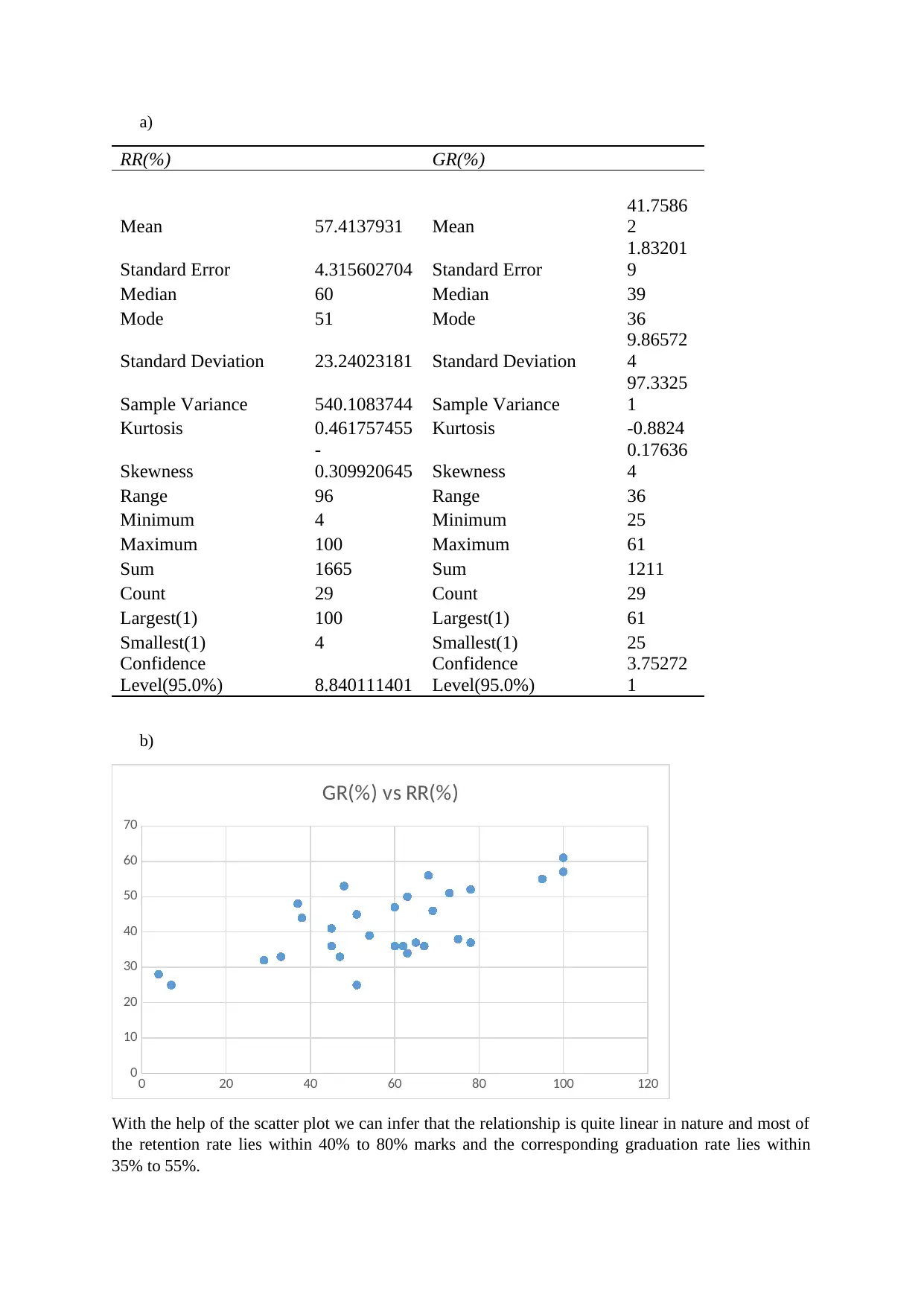
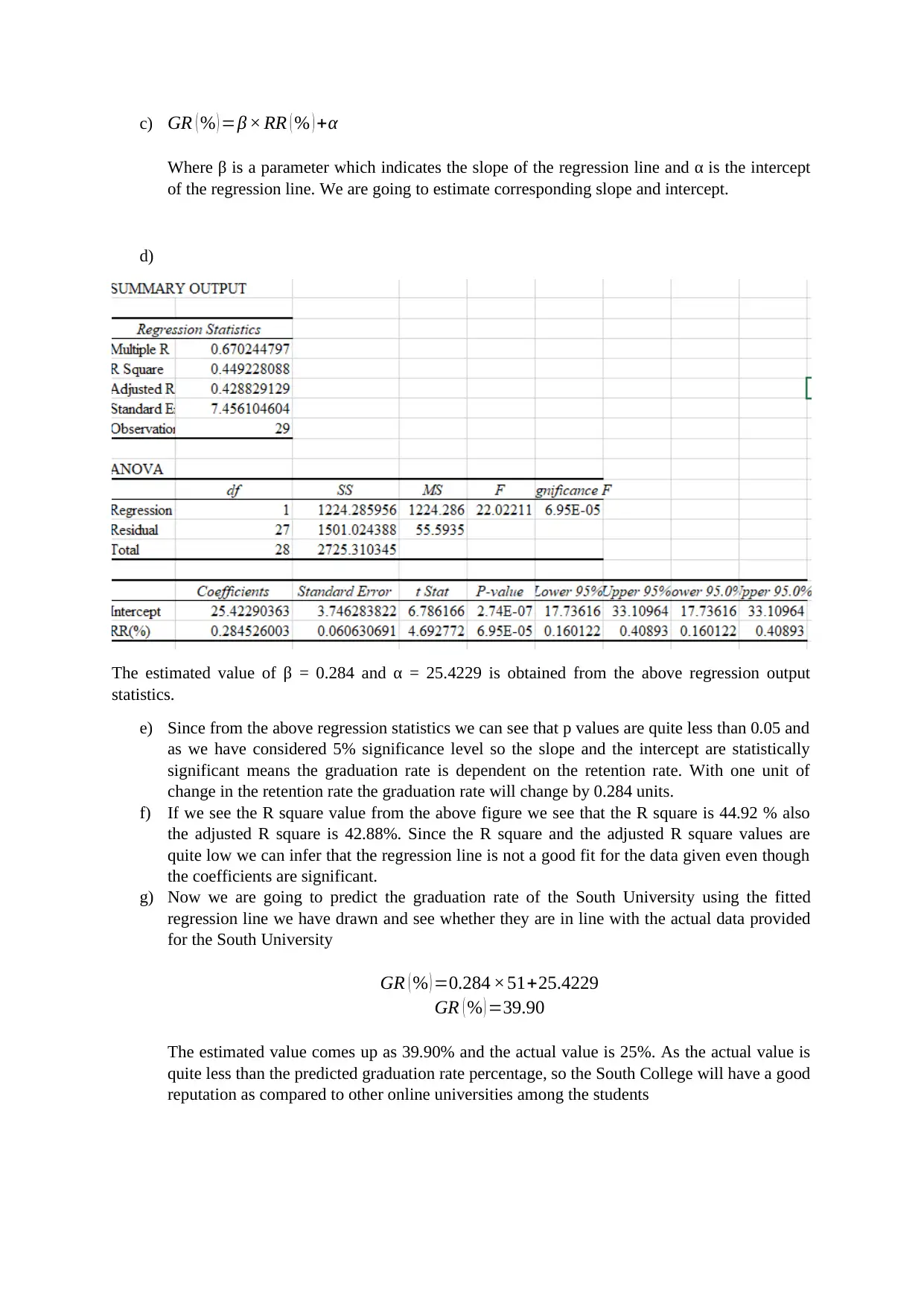
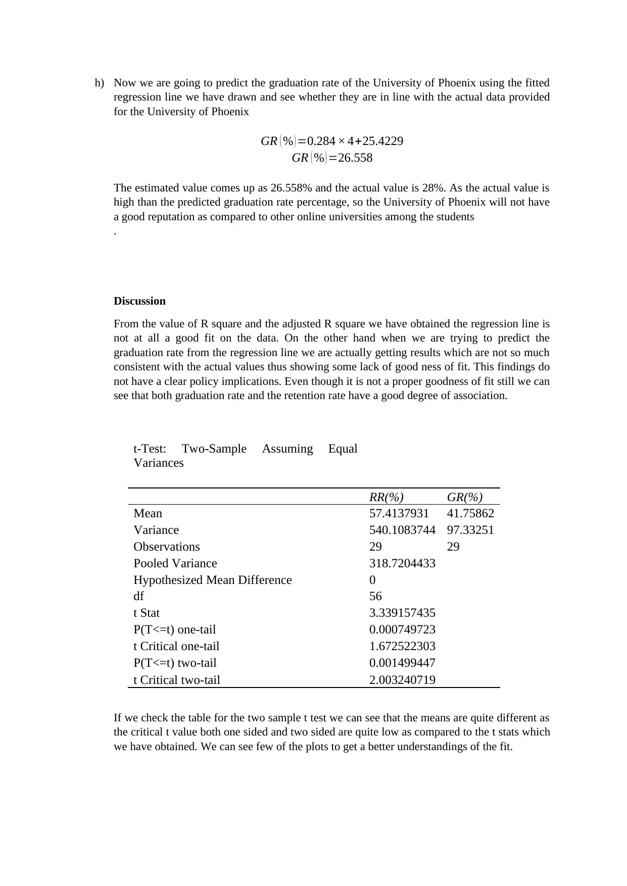
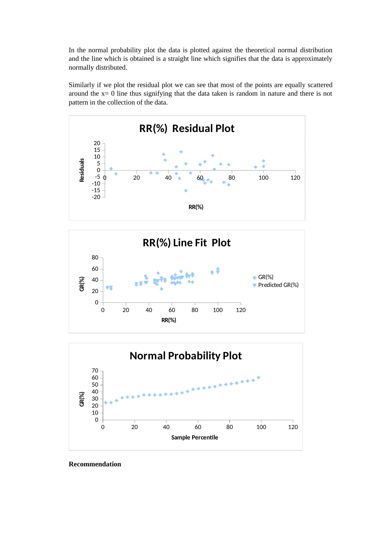
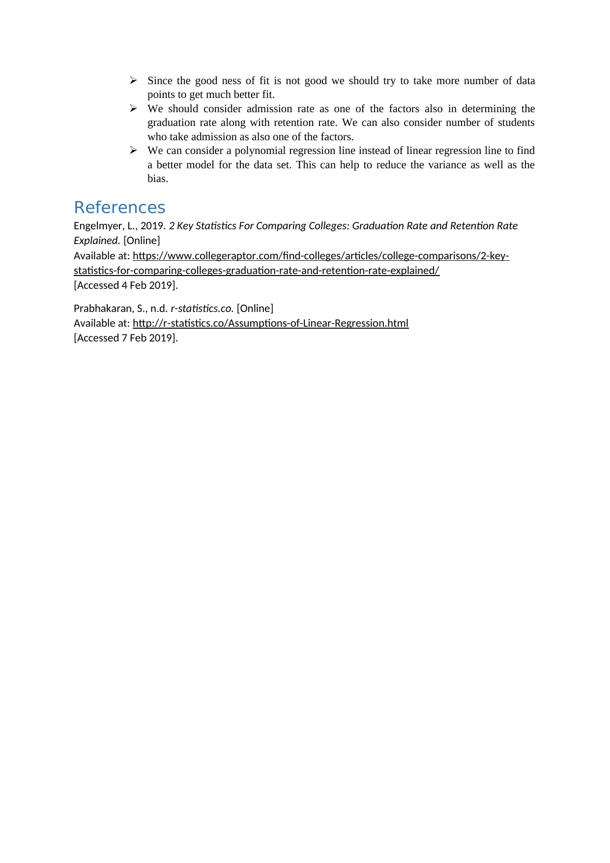
This report investigates the relationship between retention rates and graduation rates in online universities using linear regression analysis. The study begins with summary statistics for both variables, followed by fitting a regression model to the dataset. The significance of the coefficients is ass...Read More

ECONOMICS AND QUANTITATIVE
ANALYSIS
LINEAR REGRESSION REPORT

Purpose
To find out the relation between the retention rate and the association of different universities which
provides online education
Background
Graduation rates and retention rates are the criteria which is used to determine which college is best fit
foe the students. It also looks in to the decision which the students are going to take by looking in to
both these variables. The retention rate can be defined as the percentage of full-time students who
continue as a student after the graduation year. The students intends to get in to a college and gets the
graduation degree on the year they are supposed to graduate. Before spending the time and money on
a university if they get a relation between the graduation rate and the retention rate then it would be
easy for them to take the decision. Here comes the function of the economists who by their analysis
can decide in which college the students should enrol if there is an association between the graduation
rate which is the dependent variable and the retention rate which is the independent variable. To make
a substantial investment of both time and money this information are required by the economists.
What percentage of students stay with the college is determined by the retention rate and what
percentage of student finish their degree and leave the college is given by the graduation rate.
(Engelmyer, 2019)
Method
In the analysis we are first going to find out the summary statistics of both retention rate and the
graduation rate. Then we are going to fit a regression on the dataset provided i.e. to find out the
relation between graduation rate and the retention rate. The slopes or the coefficients which we
obtained from the data we are going to check significance of the coefficients of them. The sample data
which we have obtained is continuous in nature and it is not categorical also the sample taken is a
random sample which is one of the criteria for applying the linear regression model.
So there are few assumptions which we should consider while applying the linear regression:
 We assume that the relationship between the dependent and independent variable is linear in
nature. To check this we draw the scatter plot between the two data sets and see the linearity
dependence. The residual plot is also plotted once the regression line is fit in to the data to see
that the data taken is random in nature.
 we will get almost equal number of points about the line x = 0 when we are going to draw the
residual plot
 The observations provided are independent to each other.
 For any value of x the value of y varies according to a normal distribution.
 The errors are normally distributed ε ~ N (0, σ2).
 Linear relationship exists between them in a linear regression
 Multivariate normality is one of the assumptions for the model
 As there is only 1 independent variable multi collinearity won’t be a problem
 No auto-correlation or the lag term exists between the errors of the regression line
 Homoscedasticity (Prabhakaran, n.d.)
Results

a)
RR(%) GR(%)
Mean 57.4137931 Mean
41.7586
2
Standard Error 4.315602704 Standard Error
1.83201
9
Median 60 Median 39
Mode 51 Mode 36
Standard Deviation 23.24023181 Standard Deviation
9.86572
4
Sample Variance 540.1083744 Sample Variance
97.3325
1
Kurtosis 0.461757455 Kurtosis -0.8824
Skewness
-
0.309920645 Skewness
0.17636
4
Range 96 Range 36
Minimum 4 Minimum 25
Maximum 100 Maximum 61
Sum 1665 Sum 1211
Count 29 Count 29
Largest(1) 100 Largest(1) 61
Smallest(1) 4 Smallest(1) 25
Confidence
Level(95.0%) 8.840111401
Confidence
Level(95.0%)
3.75272
1
b)
0 20 40 60 80 100 120
0
10
20
30
40
50
60
70
GR(%) vs RR(%)
With the help of the scatter plot we can infer that the relationship is quite linear in nature and most of
the retention rate lies within 40% to 80% marks and the corresponding graduation rate lies within
35% to 55%.

c) GR ( % ) =β × RR ( % ) +α
Where β is a parameter which indicates the slope of the regression line and α is the intercept
of the regression line. We are going to estimate corresponding slope and intercept.
d)
The estimated value of β = 0.284 and α = 25.4229 is obtained from the above regression output
statistics.
e) Since from the above regression statistics we can see that p values are quite less than 0.05 and
as we have considered 5% significance level so the slope and the intercept are statistically
significant means the graduation rate is dependent on the retention rate. With one unit of
change in the retention rate the graduation rate will change by 0.284 units.
f) If we see the R square value from the above figure we see that the R square is 44.92 % also
the adjusted R square is 42.88%. Since the R square and the adjusted R square values are
quite low we can infer that the regression line is not a good fit for the data given even though
the coefficients are significant.
g) Now we are going to predict the graduation rate of the South University using the fitted
regression line we have drawn and see whether they are in line with the actual data provided
for the South University
GR ( % ) =0.284 ×51+25.4229
GR ( % ) =39.90
The estimated value comes up as 39.90% and the actual value is 25%. As the actual value is
quite less than the predicted graduation rate percentage, so the South College will have a good
reputation as compared to other online universities among the students

h) Now we are going to predict the graduation rate of the University of Phoenix using the fitted
regression line we have drawn and see whether they are in line with the actual data provided
for the University of Phoenix
GR ( % ) =0.284 × 4+25.4229
GR ( % ) =26.558
The estimated value comes up as 26.558% and the actual value is 28%. As the actual value is
high than the predicted graduation rate percentage, so the University of Phoenix will not have
a good reputation as compared to other online universities among the students
.
Discussion
From the value of R square and the adjusted R square we have obtained the regression line is
not at all a good fit on the data. On the other hand when we are trying to predict the
graduation rate from the regression line we are actually getting results which are not so much
consistent with the actual values thus showing some lack of good ness of fit. This findings do
not have a clear policy implications. Even though it is not a proper goodness of fit still we can
see that both graduation rate and the retention rate have a good degree of association.
t-Test: Two-Sample Assuming Equal
Variances
RR(%) GR(%)
Mean 57.4137931 41.75862
Variance 540.1083744 97.33251
Observations 29 29
Pooled Variance 318.7204433
Hypothesized Mean Difference 0
df 56
t Stat 3.339157435
P(T<=t) one-tail 0.000749723
t Critical one-tail 1.672522303
P(T<=t) two-tail 0.001499447
t Critical two-tail 2.003240719
If we check the table for the two sample t test we can see that the means are quite different as
the critical t value both one sided and two sided are quite low as compared to the t stats which
we have obtained. We can see few of the plots to get a better understandings of the fit.

In the normal probability plot the data is plotted against the theoretical normal distribution
and the line which is obtained is a straight line which signifies that the data is approximately
normally distributed.
Similarly if we plot the residual plot we can see that most of the points are equally scattered
around the x= 0 line thus signifying that the data taken is random in nature and there is not
pattern in the collection of the data.
0 20 40 60 80 100 120
-20
-15
-10
-5
0
5
10
15
20
RR(%) Residual Plot
RR(%)
Residuals
0 20 40 60 80 100 120
0
20
40
60
80
RR(%) Line Fit Plot
GR(%)
Predicted GR(%)
RR(%)
GR(%)
0 20 40 60 80 100 120
0
10
20
30
40
50
60
70
Normal Probability Plot
Sample Percentile
GR(%)
Recommendation

 Since the good ness of fit is not good we should try to take more number of data
points to get much better fit.
 We should consider admission rate as one of the factors also in determining the
graduation rate along with retention rate. We can also consider number of students
who take admission as also one of the factors.
 We can consider a polynomial regression line instead of linear regression line to find
a better model for the data set. This can help to reduce the variance as well as the
bias.
References
Engelmyer, L., 2019. 2 Key Statistics For Comparing Colleges: Graduation Rate and Retention Rate
Explained. [Online]
Available at: https://www.collegeraptor.com/find-colleges/articles/college-comparisons/2-key-
statistics-for-comparing-colleges-graduation-rate-and-retention-rate-explained/
[Accessed 4 Feb 2019].
Prabhakaran, S., n.d. r-statistics.co. [Online]
Available at: http://r-statistics.co/Assumptions-of-Linear-Regression.html
[Accessed 7 Feb 2019].