Business Economics Assignment: Analyzing Market Efficiency and Costs
VerifiedAdded on 2023/03/17
|13
|1904
|20
Homework Assignment
AI Summary
This business economics assignment delves into various aspects of market structures, including allocative efficiency under perfect and monopolistic competition, and the concepts of marginal cost and marginal product in production. It analyzes long-run average cost curves and explores constant and increasing cost industries, examining their supply curves. Furthermore, the assignment addresses market-based solutions to pollution externalities, such as taxation and tradeable pollution permits, providing a comprehensive understanding of these economic principles. Finally, the assignment includes practical applications of cost and profit analysis, offering a detailed breakdown of a firm's output, costs, and profit under different pricing scenarios.
Running head: BUSINESS ECONOMICS
Business Economics
Name of the Student
Name of the University
Student ID
Business Economics
Name of the Student
Name of the University
Student ID
Paraphrase This Document
Need a fresh take? Get an instant paraphrase of this document with our AI Paraphraser
1BUSINESS ECONOMICS
Table of Contents
Answer 2....................................................................................................................................2
Answer a.................................................................................................................................2
Answer b................................................................................................................................3
Answer 3....................................................................................................................................4
Answer a.................................................................................................................................4
Answer b................................................................................................................................5
Answer c.................................................................................................................................6
Answer 5....................................................................................................................................6
Answer 6....................................................................................................................................8
Answer 8..................................................................................................................................10
Answer a...............................................................................................................................10
Answer b..............................................................................................................................10
Answer c...............................................................................................................................10
Answer d..............................................................................................................................10
Answer e...............................................................................................................................10
Answer f...............................................................................................................................11
Answer g..............................................................................................................................11
Answer h..............................................................................................................................11
Answer i...............................................................................................................................11
References................................................................................................................................12
2BUSINESS ECONOMICS
Answer 2
Answer a
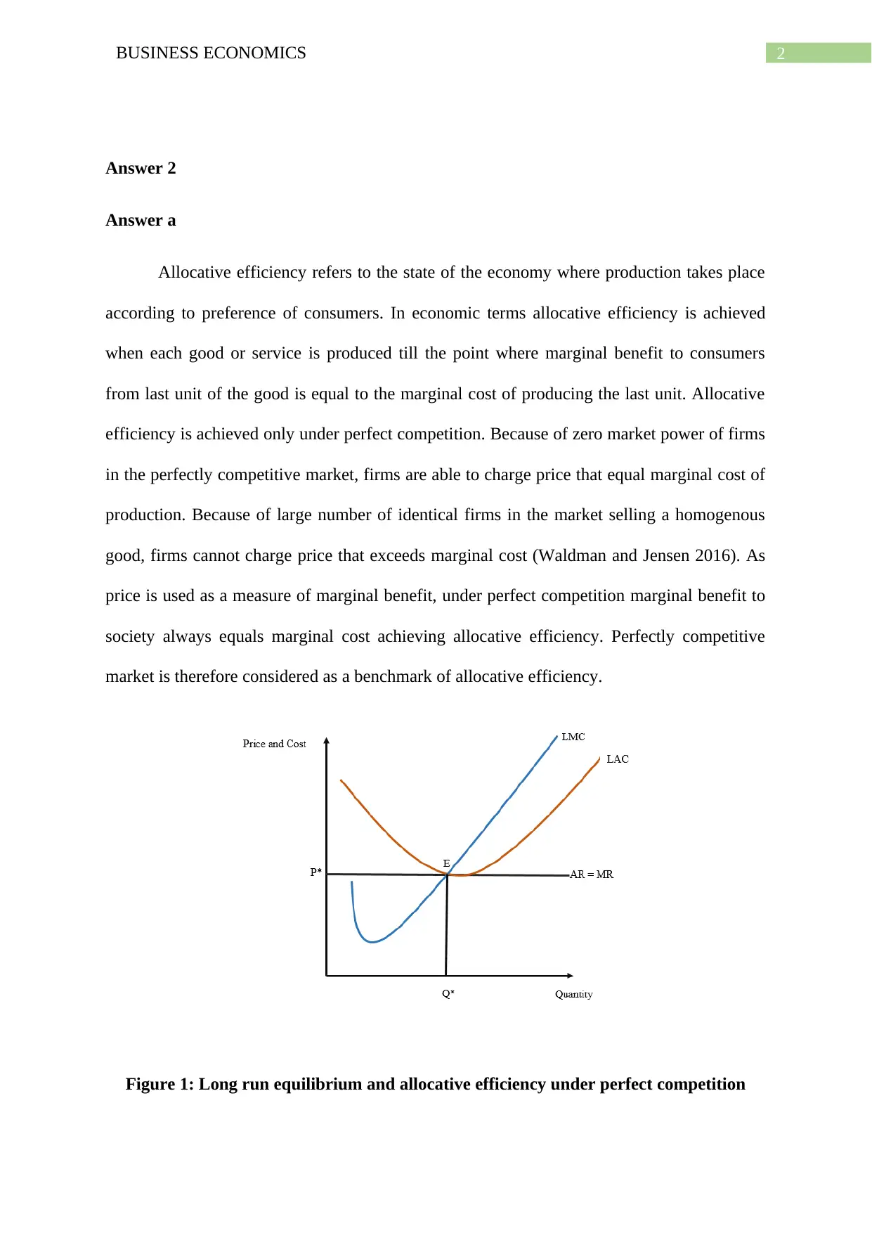
Allocative efficiency refers to the state of the economy where production takes place
according to preference of consumers. In economic terms allocative efficiency is achieved
when each good or service is produced till the point where marginal benefit to consumers
from last unit of the good is equal to the marginal cost of producing the last unit. Allocative
efficiency is achieved only under perfect competition. Because of zero market power of firms
in the perfectly competitive market, firms are able to charge price that equal marginal cost of
production. Because of large number of identical firms in the market selling a homogenous
good, firms cannot charge price that exceeds marginal cost (Waldman and Jensen 2016). As
price is used as a measure of marginal benefit, under perfect competition marginal benefit to
society always equals marginal cost achieving allocative efficiency. Perfectly competitive
market is therefore considered as a benchmark of allocative efficiency.
Figure 1: Long run equilibrium and allocative efficiency under perfect competition
Answer 2
Answer a
Allocative efficiency refers to the state of the economy where production takes place
according to preference of consumers. In economic terms allocative efficiency is achieved
when each good or service is produced till the point where marginal benefit to consumers
from last unit of the good is equal to the marginal cost of producing the last unit. Allocative
efficiency is achieved only under perfect competition. Because of zero market power of firms
in the perfectly competitive market, firms are able to charge price that equal marginal cost of
production. Because of large number of identical firms in the market selling a homogenous
good, firms cannot charge price that exceeds marginal cost (Waldman and Jensen 2016). As
price is used as a measure of marginal benefit, under perfect competition marginal benefit to
society always equals marginal cost achieving allocative efficiency. Perfectly competitive
market is therefore considered as a benchmark of allocative efficiency.
Figure 1: Long run equilibrium and allocative efficiency under perfect competition
⊘ This is a preview!⊘
Do you want full access?
Subscribe today to unlock all pages.
Trusted by 1+ million students worldwide
3BUSINESS ECONOMICS
Answer b
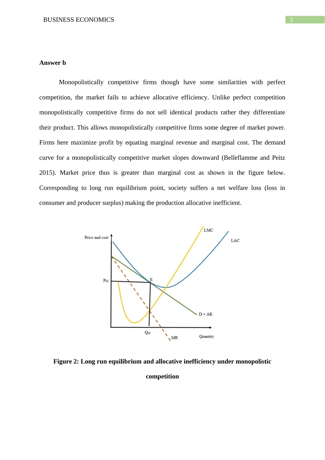
Monopolistically competitive firms though have some similarities with perfect
competition, the market fails to achieve allocative efficiency. Unlike perfect competition
monopolistically competitive firms do not sell identical products rather they differentiate
their product. This allows monopolistically competitive firms some degree of market power.
Firms here maximize profit by equating marginal revenue and marginal cost. The demand
curve for a monopolistically competitive market slopes downward (Belleflamme and Peitz
2015). Market price thus is greater than marginal cost as shown in the figure below.
Corresponding to long run equilibrium point, society suffers a net welfare loss (loss in
consumer and producer surplus) making the production allocative inefficient.
Figure 2: Long run equilibrium and allocative inefficiency under monopolistic
competition
Answer b
Monopolistically competitive firms though have some similarities with perfect
competition, the market fails to achieve allocative efficiency. Unlike perfect competition
monopolistically competitive firms do not sell identical products rather they differentiate
their product. This allows monopolistically competitive firms some degree of market power.
Firms here maximize profit by equating marginal revenue and marginal cost. The demand
curve for a monopolistically competitive market slopes downward (Belleflamme and Peitz
2015). Market price thus is greater than marginal cost as shown in the figure below.
Corresponding to long run equilibrium point, society suffers a net welfare loss (loss in
consumer and producer surplus) making the production allocative inefficient.
Figure 2: Long run equilibrium and allocative inefficiency under monopolistic
competition
Paraphrase This Document
Need a fresh take? Get an instant paraphrase of this document with our AI Paraphraser
4BUSINESS ECONOMICS
Answer 3
Answer a
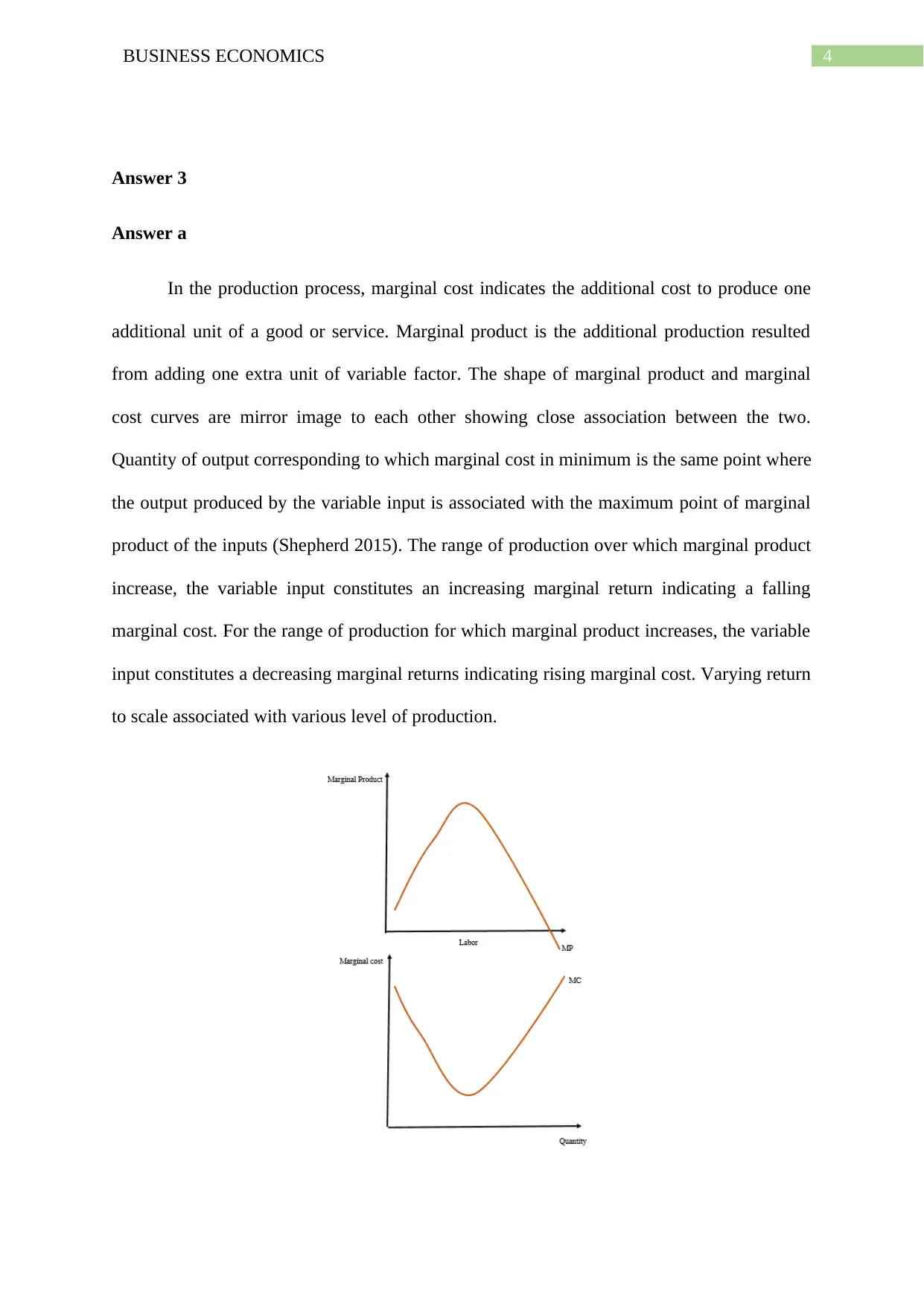
In the production process, marginal cost indicates the additional cost to produce one
additional unit of a good or service. Marginal product is the additional production resulted
from adding one extra unit of variable factor. The shape of marginal product and marginal
cost curves are mirror image to each other showing close association between the two.
Quantity of output corresponding to which marginal cost in minimum is the same point where
the output produced by the variable input is associated with the maximum point of marginal
product of the inputs (Shepherd 2015). The range of production over which marginal product
increase, the variable input constitutes an increasing marginal return indicating a falling
marginal cost. For the range of production for which marginal product increases, the variable
input constitutes a decreasing marginal returns indicating rising marginal cost. Varying return
to scale associated with various level of production.
Answer 3
Answer a
In the production process, marginal cost indicates the additional cost to produce one
additional unit of a good or service. Marginal product is the additional production resulted
from adding one extra unit of variable factor. The shape of marginal product and marginal
cost curves are mirror image to each other showing close association between the two.
Quantity of output corresponding to which marginal cost in minimum is the same point where
the output produced by the variable input is associated with the maximum point of marginal
product of the inputs (Shepherd 2015). The range of production over which marginal product
increase, the variable input constitutes an increasing marginal return indicating a falling
marginal cost. For the range of production for which marginal product increases, the variable
input constitutes a decreasing marginal returns indicating rising marginal cost. Varying return
to scale associated with various level of production.
5BUSINESS ECONOMICS
Figure 3: Marginal cost and marginal product
Answer b
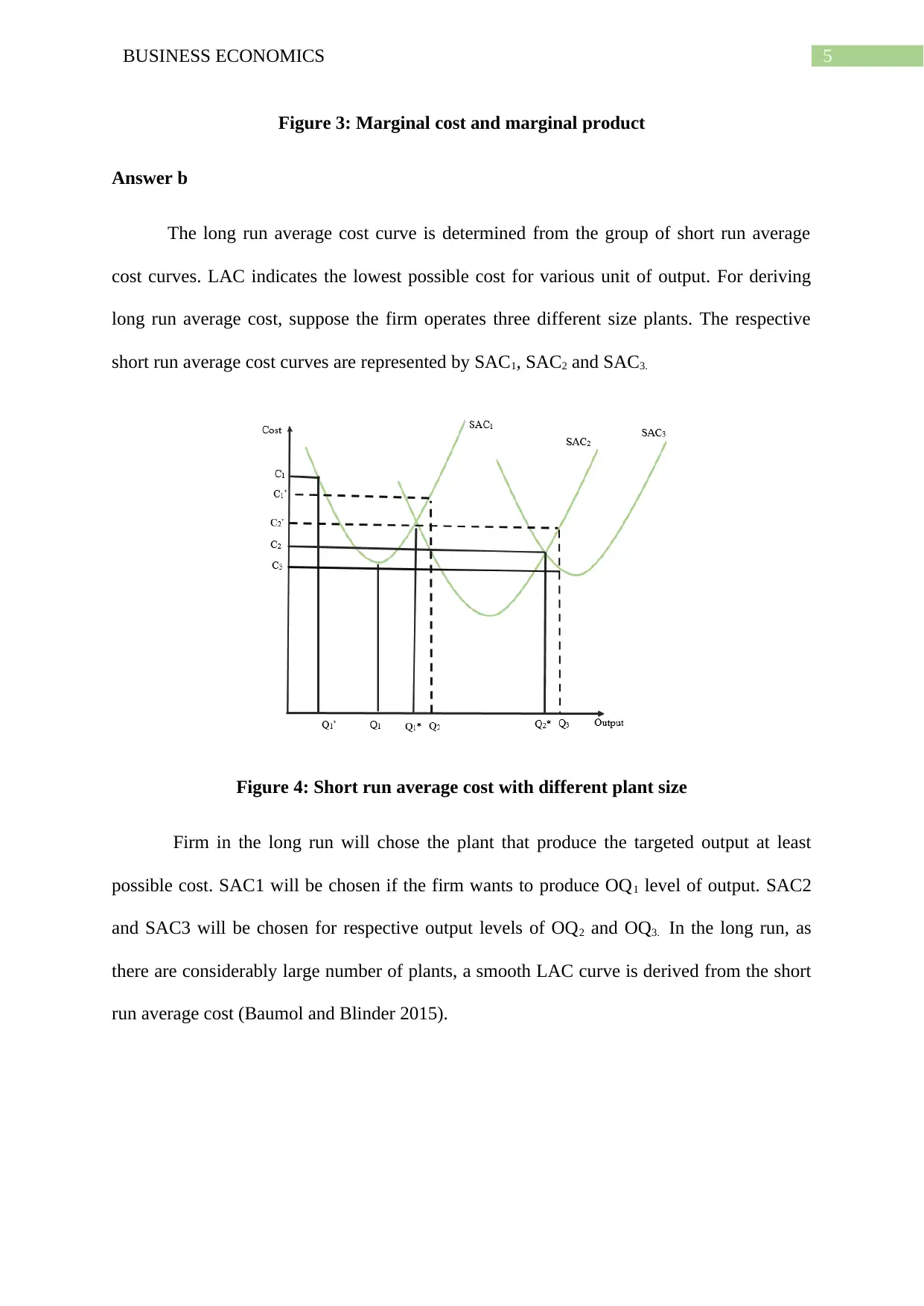
The long run average cost curve is determined from the group of short run average
cost curves. LAC indicates the lowest possible cost for various unit of output. For deriving
long run average cost, suppose the firm operates three different size plants. The respective
short run average cost curves are represented by SAC1, SAC2 and SAC3.
Figure 4: Short run average cost with different plant size
Firm in the long run will chose the plant that produce the targeted output at least
possible cost. SAC1 will be chosen if the firm wants to produce OQ1 level of output. SAC2
and SAC3 will be chosen for respective output levels of OQ2 and OQ3. In the long run, as
there are considerably large number of plants, a smooth LAC curve is derived from the short
run average cost (Baumol and Blinder 2015).
Figure 3: Marginal cost and marginal product
Answer b
The long run average cost curve is determined from the group of short run average
cost curves. LAC indicates the lowest possible cost for various unit of output. For deriving
long run average cost, suppose the firm operates three different size plants. The respective
short run average cost curves are represented by SAC1, SAC2 and SAC3.
Figure 4: Short run average cost with different plant size
Firm in the long run will chose the plant that produce the targeted output at least
possible cost. SAC1 will be chosen if the firm wants to produce OQ1 level of output. SAC2
and SAC3 will be chosen for respective output levels of OQ2 and OQ3. In the long run, as
there are considerably large number of plants, a smooth LAC curve is derived from the short
run average cost (Baumol and Blinder 2015).
⊘ This is a preview!⊘
Do you want full access?
Subscribe today to unlock all pages.
Trusted by 1+ million students worldwide
6BUSINESS ECONOMICS
Figure 5: Long run average cost curve
Answer c
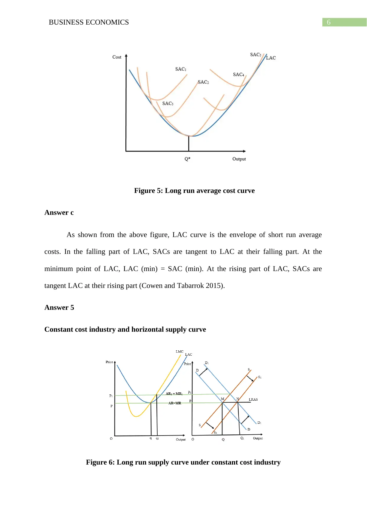
As shown from the above figure, LAC curve is the envelope of short run average
costs. In the falling part of LAC, SACs are tangent to LAC at their falling part. At the
minimum point of LAC, LAC (min) = SAC (min). At the rising part of LAC, SACs are
tangent LAC at their rising part (Cowen and Tabarrok 2015).
Answer 5
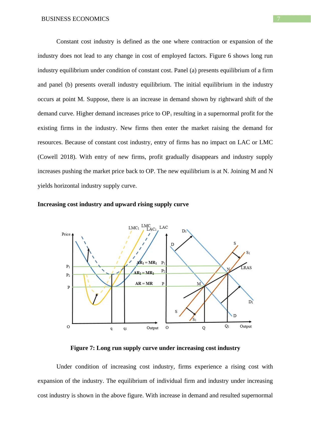
Constant cost industry and horizontal supply curve
Figure 6: Long run supply curve under constant cost industry
Figure 5: Long run average cost curve
Answer c
As shown from the above figure, LAC curve is the envelope of short run average
costs. In the falling part of LAC, SACs are tangent to LAC at their falling part. At the
minimum point of LAC, LAC (min) = SAC (min). At the rising part of LAC, SACs are
tangent LAC at their rising part (Cowen and Tabarrok 2015).
Answer 5
Constant cost industry and horizontal supply curve
Figure 6: Long run supply curve under constant cost industry
Paraphrase This Document
Need a fresh take? Get an instant paraphrase of this document with our AI Paraphraser
7BUSINESS ECONOMICS
Constant cost industry is defined as the one where contraction or expansion of the
industry does not lead to any change in cost of employed factors. Figure 6 shows long run
industry equilibrium under condition of constant cost. Panel (a) presents equilibrium of a firm
and panel (b) presents overall industry equilibrium. The initial equilibrium in the industry
occurs at point M. Suppose, there is an increase in demand shown by rightward shift of the
demand curve. Higher demand increases price to OP1 resulting in a supernormal profit for the
existing firms in the industry. New firms then enter the market raising the demand for
resources. Because of constant cost industry, entry of firms has no impact on LAC or LMC
(Cowell 2018). With entry of new firms, profit gradually disappears and industry supply
increases pushing the market price back to OP. The new equilibrium is at N. Joining M and N
yields horizontal industry supply curve.
Increasing cost industry and upward rising supply curve
Figure 7: Long run supply curve under increasing cost industry
Under condition of increasing cost industry, firms experience a rising cost with
expansion of the industry. The equilibrium of individual firm and industry under increasing
cost industry is shown in the above figure. With increase in demand and resulted supernormal
8BUSINESS ECONOMICS
profit new firms enter the industry. As a result, resource demand increases causing input price
to increase (increasing cost industry) (Mankiw 2014). This shift the cost curves upward.
Because of increased cost firms’ supply do not extend that much as in case of constant cost
industry. The supply curve shifts rightward to S1S1. OQ1 quantity is now supplied at price
OP2. Joining M and new equilibrium N gives an upward sloping industry supply curve.
Answer 6
Market based solution to pollution externality
Pollution is a form of negative externality producing socially inefficient outcome.
Two market based approach to solve the problem of pollution externality are tax and
tradeable pollution permits.
Tax
For production activities creating pollution, marginal social cost exceeds the marginal
private cost. This results in over production of the particular good. In order to internalize the
externality a tax should be imposed equivalent to the external cost. Taxing polluting activities
is a market based approach that estimates maximum costs for controlling measures (Friedman
2017). The provides polluters an incentive to lower pollution at a cheaper rate than tax. The
quantity of pollution depends on the tax rate.
⊘ This is a preview!⊘
Do you want full access?
Subscribe today to unlock all pages.
Trusted by 1+ million students worldwide
9BUSINESS ECONOMICS
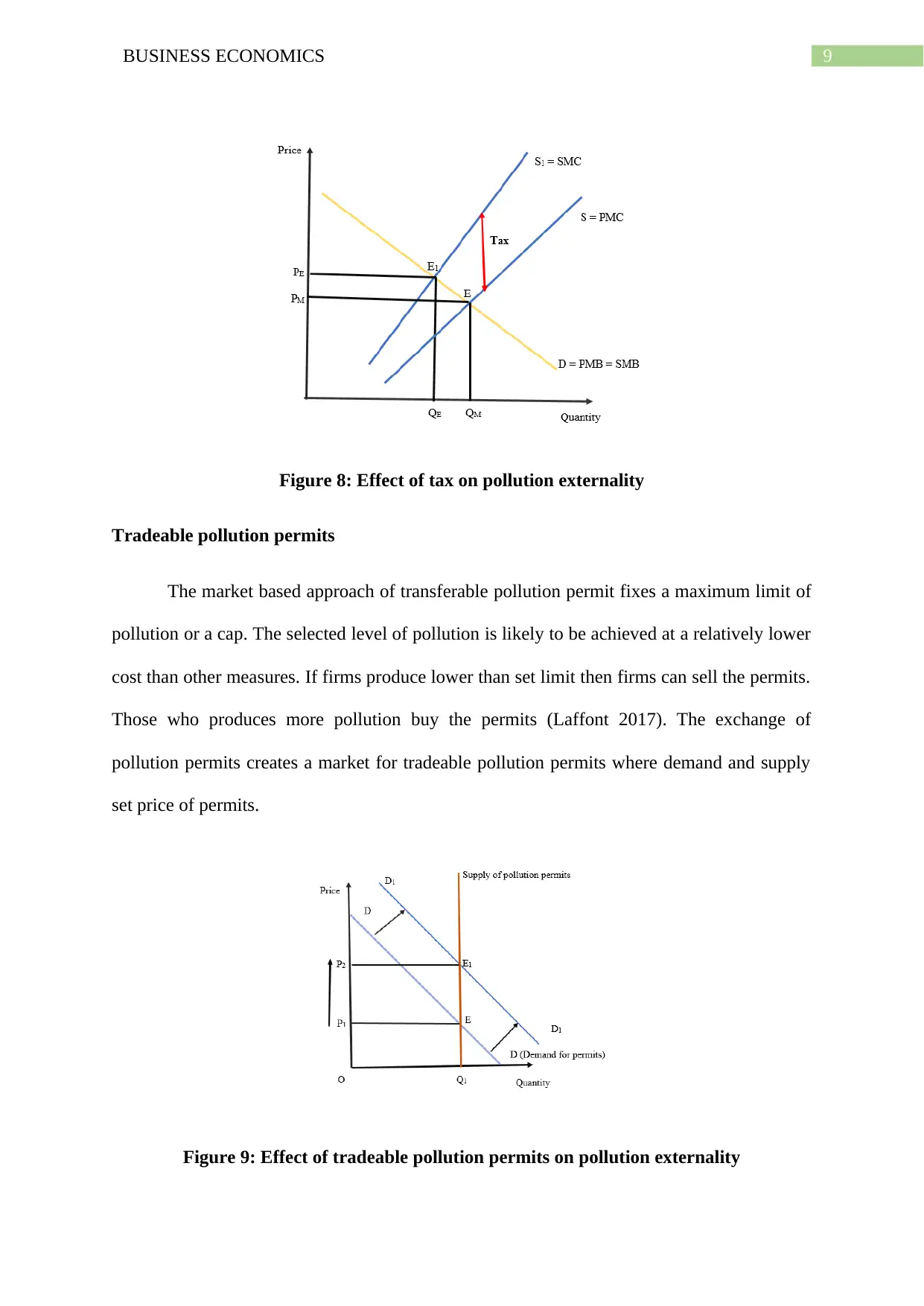
Figure 8: Effect of tax on pollution externality
Tradeable pollution permits
The market based approach of transferable pollution permit fixes a maximum limit of
pollution or a cap. The selected level of pollution is likely to be achieved at a relatively lower
cost than other measures. If firms produce lower than set limit then firms can sell the permits.
Those who produces more pollution buy the permits (Laffont 2017). The exchange of
pollution permits creates a market for tradeable pollution permits where demand and supply
set price of permits.
Figure 9: Effect of tradeable pollution permits on pollution externality
Paraphrase This Document
Need a fresh take? Get an instant paraphrase of this document with our AI Paraphraser
10BUSINESS ECONOMICS
Answer 8
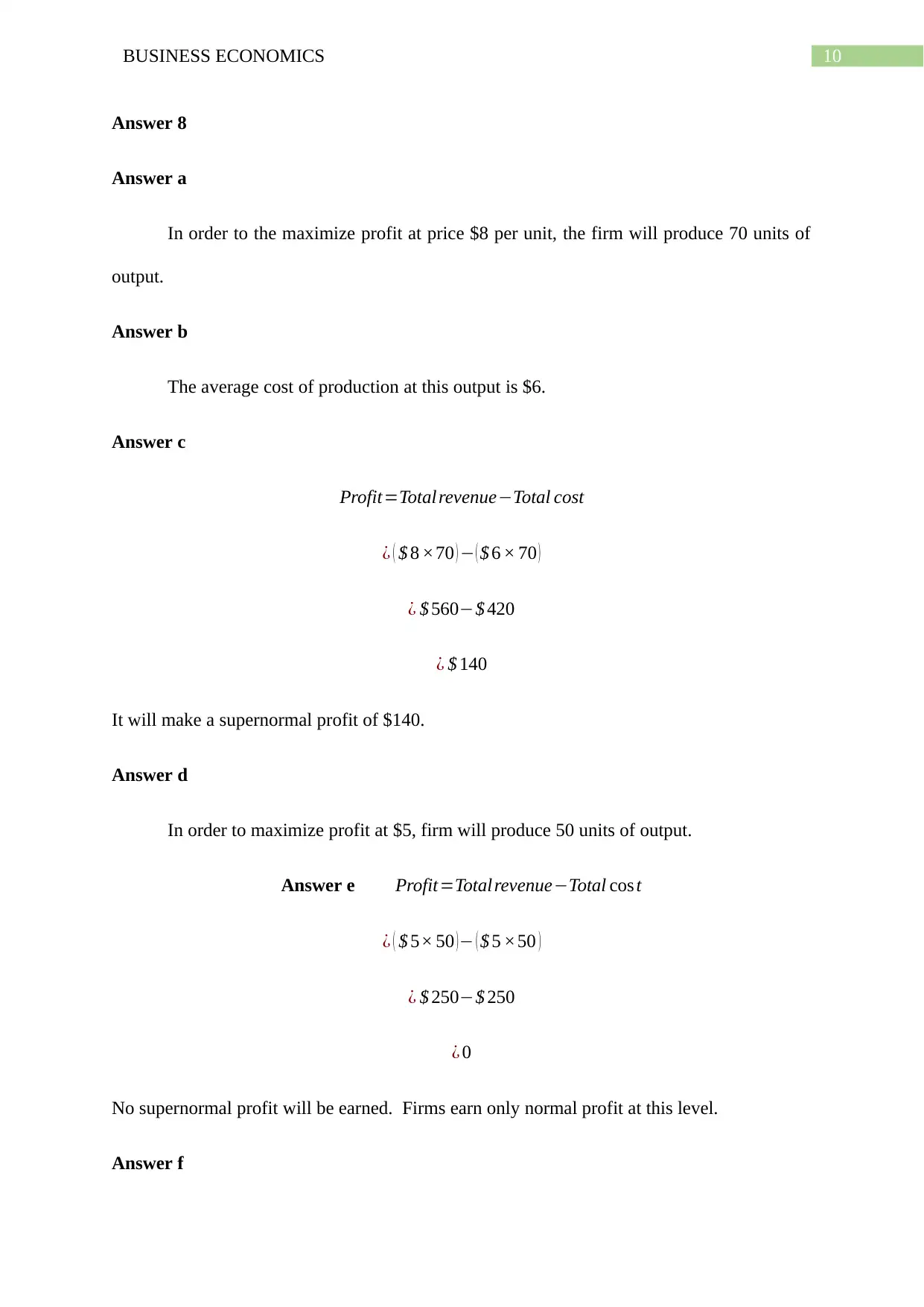
Answer a
In order to the maximize profit at price $8 per unit, the firm will produce 70 units of
output.
Answer b
The average cost of production at this output is $6.
Answer c
Profit=Total revenue−Total cost
¿ ( $ 8 ×70 ) − ( $ 6 × 70 )
¿ $ 560−$ 420
¿ $ 140
It will make a supernormal profit of $140.
Answer d
In order to maximize profit at $5, firm will produce 50 units of output.
Answer e Profit=Total revenue−Total cos t
¿ ( $ 5× 50 )− ( $ 5 ×50 )
¿ $ 250−$ 250
¿ 0
No supernormal profit will be earned. Firms earn only normal profit at this level.
Answer f
Answer 8
Answer a
In order to the maximize profit at price $8 per unit, the firm will produce 70 units of
output.
Answer b
The average cost of production at this output is $6.
Answer c
Profit=Total revenue−Total cost
¿ ( $ 8 ×70 ) − ( $ 6 × 70 )
¿ $ 560−$ 420
¿ $ 140
It will make a supernormal profit of $140.
Answer d
In order to maximize profit at $5, firm will produce 50 units of output.
Answer e Profit=Total revenue−Total cos t
¿ ( $ 5× 50 )− ( $ 5 ×50 )
¿ $ 250−$ 250
¿ 0
No supernormal profit will be earned. Firms earn only normal profit at this level.
Answer f
11BUSINESS ECONOMICS
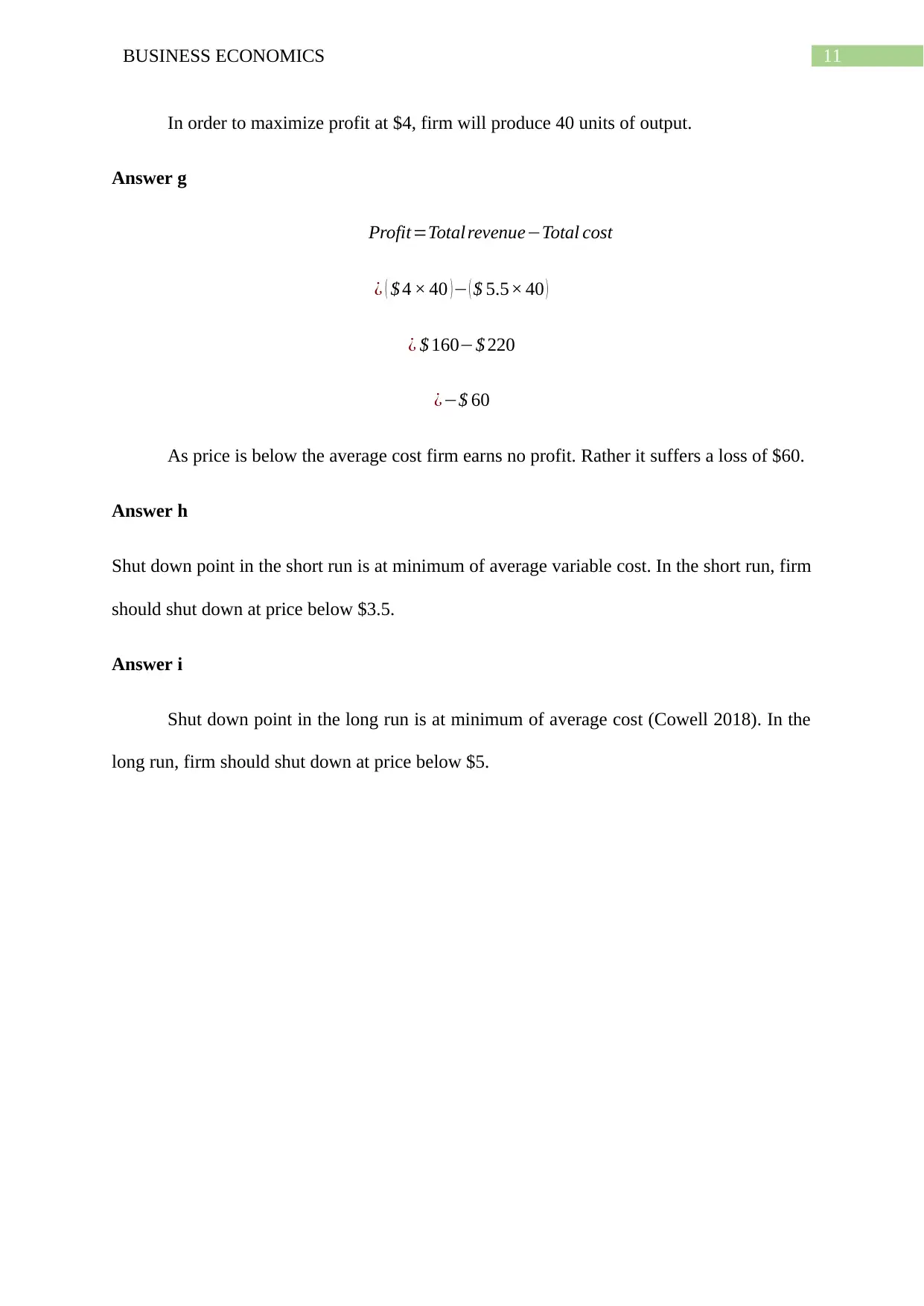
In order to maximize profit at $4, firm will produce 40 units of output.
Answer g
Profit=Total revenue−Total cost
¿ ( $ 4 × 40 )− ( $ 5.5× 40 )
¿ $ 160−$ 220
¿−$ 60
As price is below the average cost firm earns no profit. Rather it suffers a loss of $60.
Answer h
Shut down point in the short run is at minimum of average variable cost. In the short run, firm
should shut down at price below $3.5.
Answer i
Shut down point in the long run is at minimum of average cost (Cowell 2018). In the
long run, firm should shut down at price below $5.
⊘ This is a preview!⊘
Do you want full access?
Subscribe today to unlock all pages.
Trusted by 1+ million students worldwide
1 out of 13
Related Documents


Your All-in-One AI-Powered Toolkit for Academic Success.
+13062052269
info@desklib.com
Available 24*7 on WhatsApp / Email
![[object Object]](/_next/static/media/star-bottom.7253800d.svg)
Unlock your academic potential
Copyright © 2020–2026 A2Z Services. All Rights Reserved. Developed and managed by ZUCOL.