EDU10447 S1 2018: Statistical Analysis and Real-World Relevance

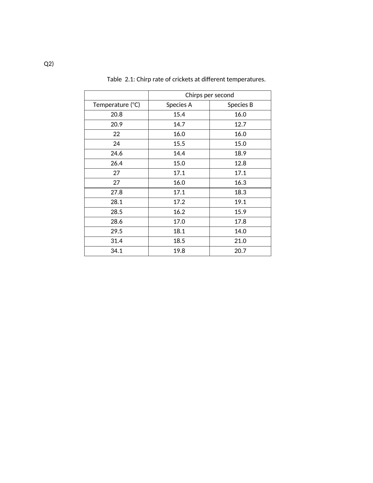
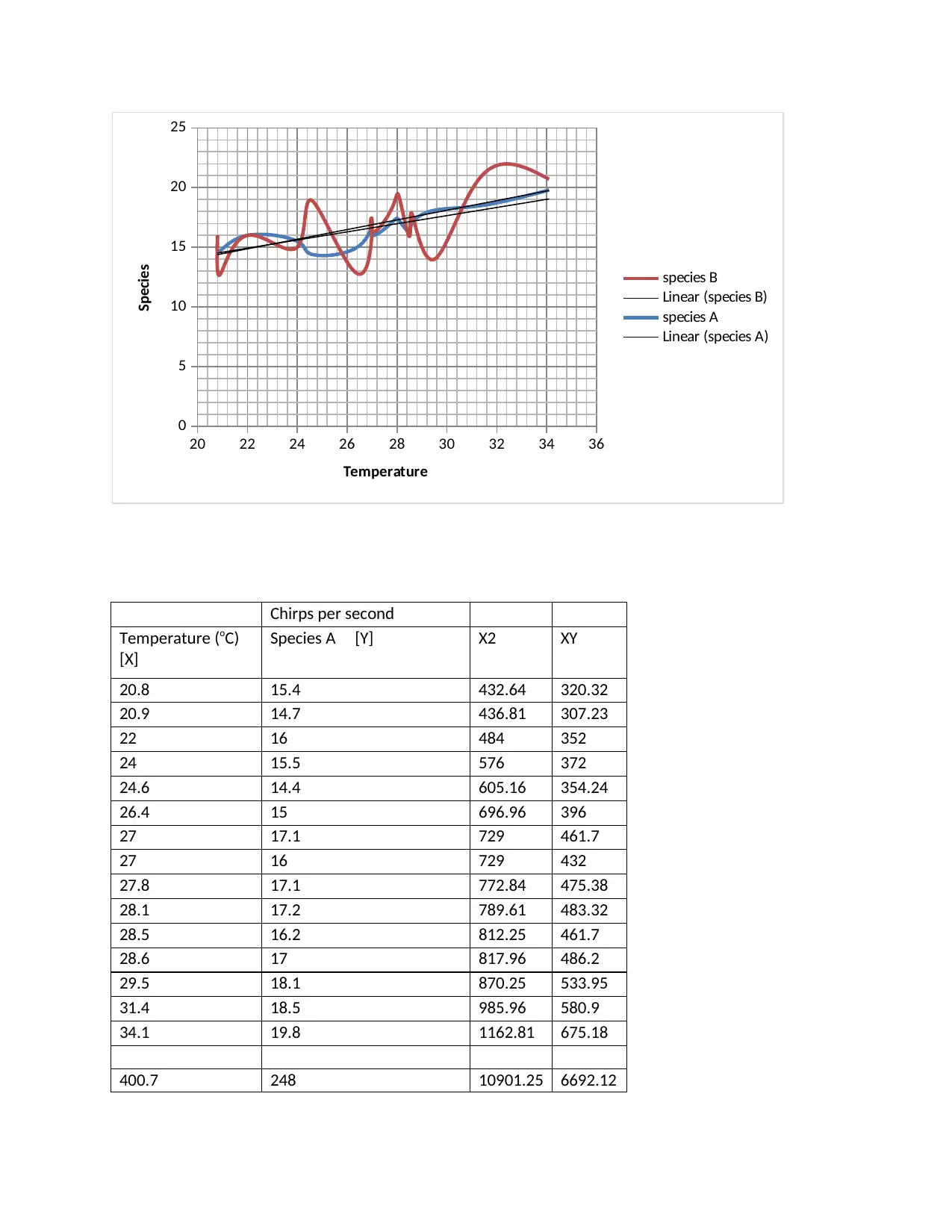
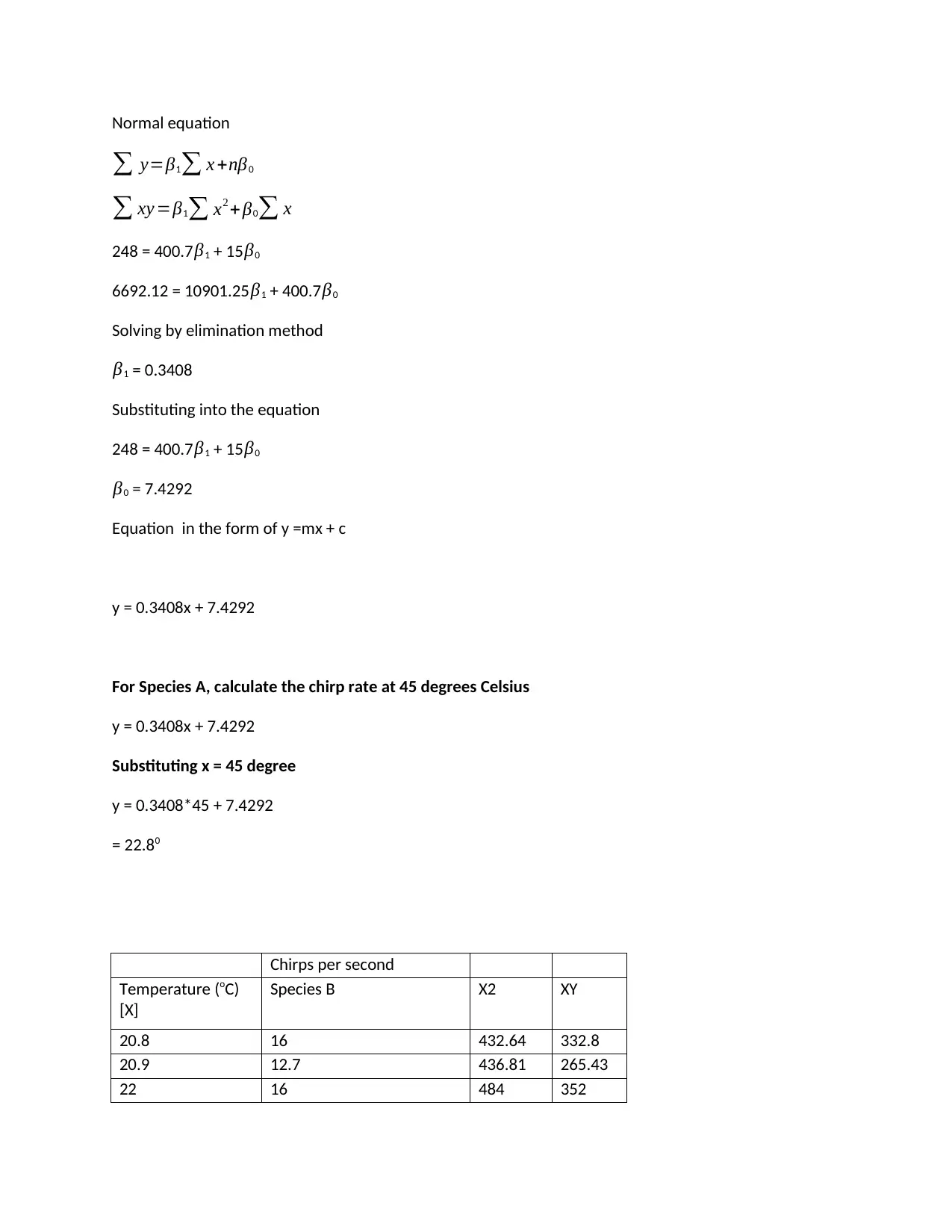
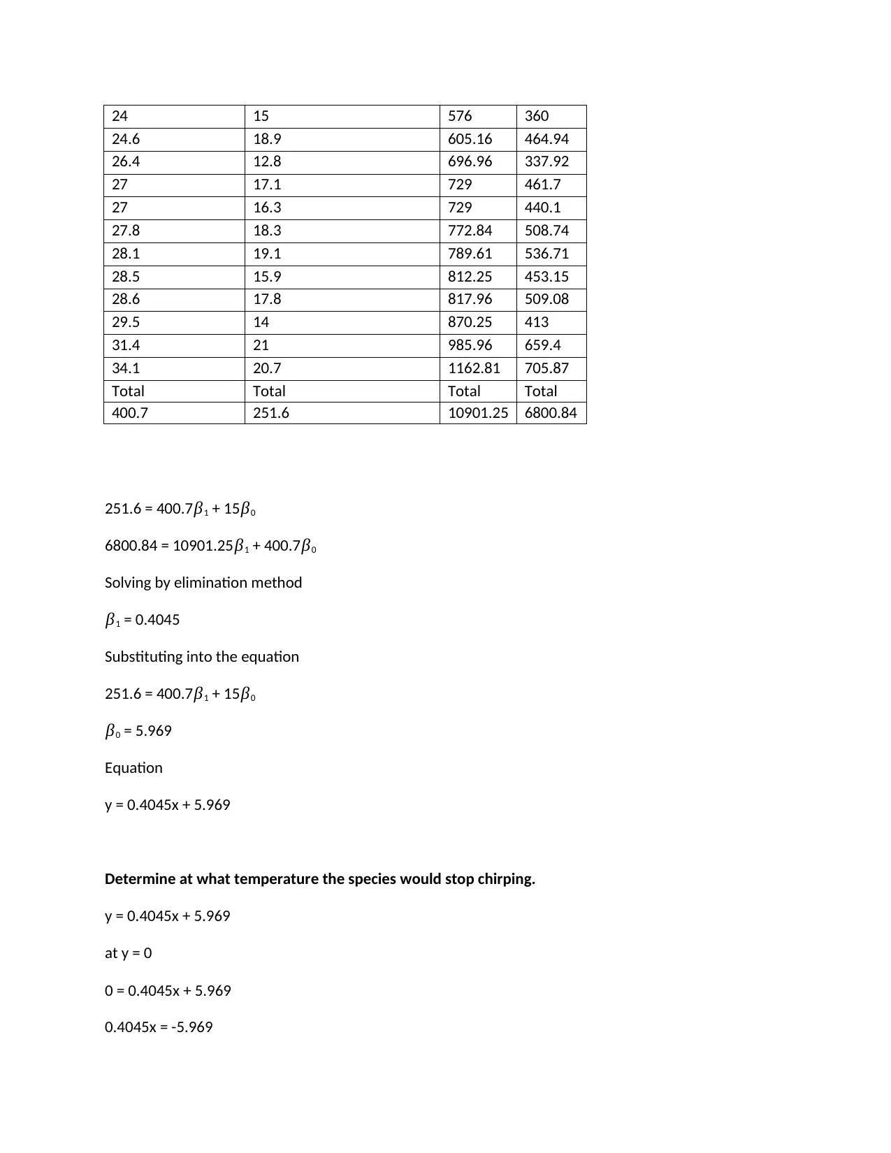
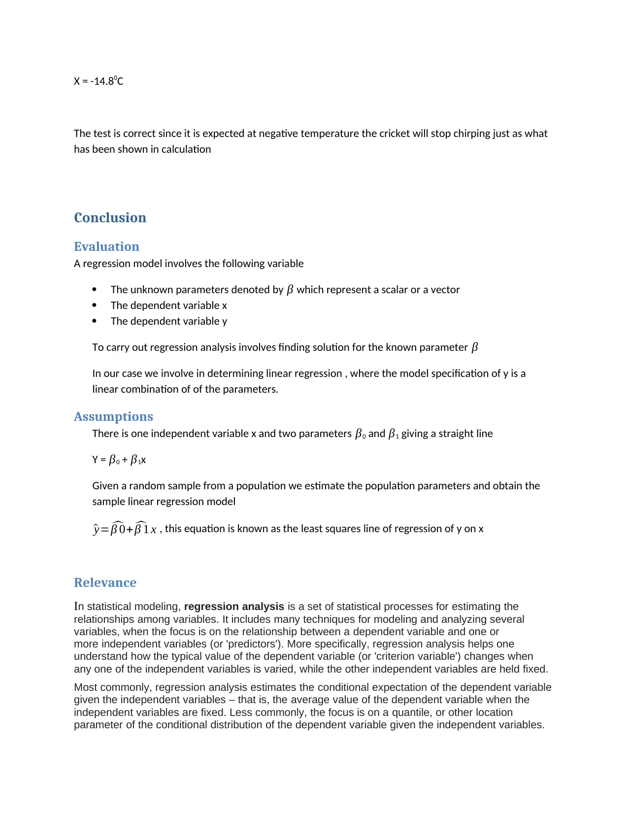
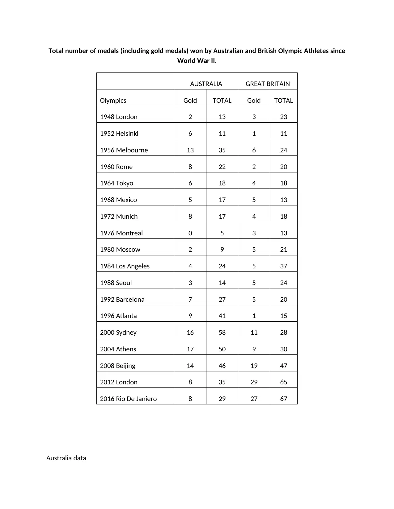
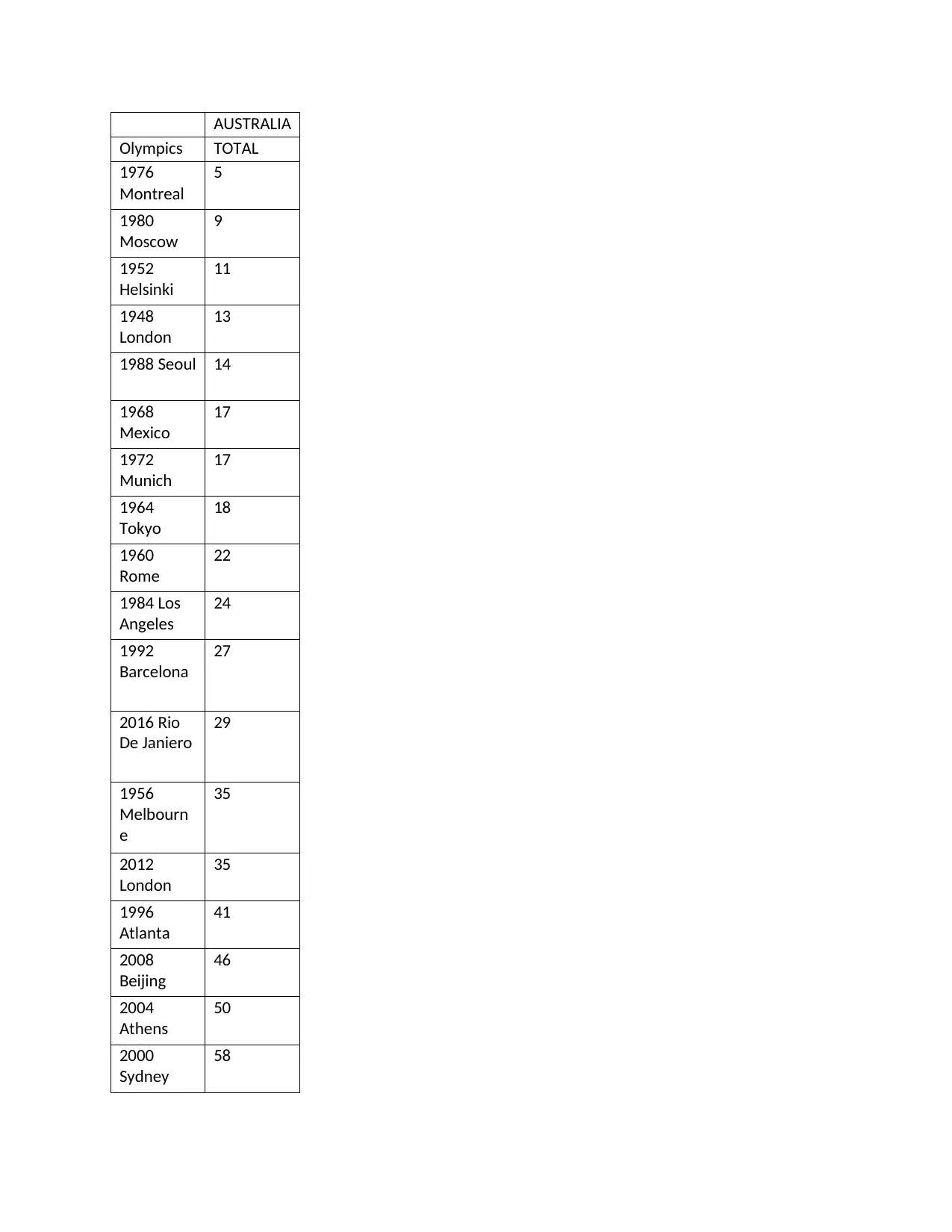
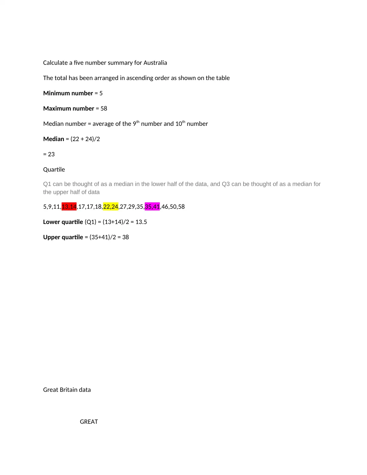
This assignment provides solutions to three statistical problems. The first problem involves calculating the area of two sites using complete and incomplete squares and applying a scale factor. The second problem uses linear regression to analyze the chirp rate of crickets at different temperatures for two species, including determining the chirp rate at 45 degrees Celsius and the temperature at which chirping stops. The third problem calculates a five-number summary (minimum, maximum, median, lower quartile, and upper quartile) for the total number of medals won by Australian and British Olympic athletes since World War II, along with calculating the mean for both countries. The assignment includes evaluations, assumptions, and relevance to real-world applications for each problem.

Q1)
Site 1
Area of Complete squares = 138 cm2
Area of Incomplete squares = 40/2 = 20cm2
Total area = 158 m2
But the scale = 1: 40 000
Actual area = 158 * 40000 *40000 = 2.528 *1011 cm2
But,
1Km2 = 100000cm * 100000 cm

1Km2 = 10000000000 cm2
2.528 *1011 cm2
= 25.28 km2
Site 2
Area of Complete squares = 119 cm2
Area of Incomplete squares = 70/2 = 35cm2
Total area = 154 m2
But the scale = 1: 40 000

Actual area = 154 * 40000 *40000 = 2.464 *1011 cm2
But,
1Km2 = 100000cm * 100000 cm
1Km2 = 10000000000 cm2
2.464 *1011 cm2
= 24.64 km2
Conclusion
Evaluation
The calculation of the area of the sites involves subdividing the area using equal squares of dimension of
1 cm, where the incomplete squares covered will be divided by two and added to the total number of
complete squares, the total will then be multiply by area of one square since they are similar to
determine the total surface area covered, after which it will be multiplied by the scale to determine the
actual area then it will be converted to square kilometers.
Assumption
1. The square are equal and have a dimensions of 1 cm
2. The incomplete squares are made complete by dividing their total number by 2
Relevance to real world
The surveyors and architectures will use this method in drawing their plan and also interpreting it, to
easily help to determine the surface area of a particular land or area to be covered with a building
respectively.

Q2)
Table 2.1: Chirp rate of crickets at different temperatures.
Chirps per second
Temperature (oC) Species A Species B
20.8 15.4 16.0
20.9 14.7 12.7
22 16.0 16.0
24 15.5 15.0
24.6 14.4 18.9
26.4 15.0 12.8
27 17.1 17.1
27 16.0 16.3
27.8 17.1 18.3
28.1 17.2 19.1
28.5 16.2 15.9
28.6 17.0 17.8
29.5 18.1 14.0
31.4 18.5 21.0
34.1 19.8 20.7

20 22 24 26 28 30 32 34 36
0
5
10
15
20
25
species B
Linear (species B)
species A
Linear (species A)
Temperature
Species
Chirps per second
Temperature (oC)
[X]
Species A [Y] X2 XY
20.8 15.4 432.64 320.32
20.9 14.7 436.81 307.23
22 16 484 352
24 15.5 576 372
24.6 14.4 605.16 354.24
26.4 15 696.96 396
27 17.1 729 461.7
27 16 729 432
27.8 17.1 772.84 475.38
28.1 17.2 789.61 483.32
28.5 16.2 812.25 461.7
28.6 17 817.96 486.2
29.5 18.1 870.25 533.95
31.4 18.5 985.96 580.9
34.1 19.8 1162.81 675.18
400.7 248 10901.25 6692.12

Normal equation
∑ y=β1∑ x +nβ0
∑ xy =β1∑ x2 + β0∑ x
248 = 400.7 β1 + 15β0
6692.12 = 10901.25 β1 + 400.7 β0
Solving by elimination method
β1 = 0.3408
Substituting into the equation
248 = 400.7 β1 + 15 β0
β0 = 7.4292
Equation in the form of y =mx + c
y = 0.3408x + 7.4292
For Species A, calculate the chirp rate at 45 degrees Celsius
y = 0.3408x + 7.4292
Substituting x = 45 degree
y = 0.3408*45 + 7.4292
= 22.80
Chirps per second
Temperature (oC)
[X]
Species B X2 XY
20.8 16 432.64 332.8
20.9 12.7 436.81 265.43
22 16 484 352

24 15 576 360
24.6 18.9 605.16 464.94
26.4 12.8 696.96 337.92
27 17.1 729 461.7
27 16.3 729 440.1
27.8 18.3 772.84 508.74
28.1 19.1 789.61 536.71
28.5 15.9 812.25 453.15
28.6 17.8 817.96 509.08
29.5 14 870.25 413
31.4 21 985.96 659.4
34.1 20.7 1162.81 705.87
Total Total Total Total
400.7 251.6 10901.25 6800.84
251.6 = 400.7β1 + 15 β0
6800.84 = 10901.25 β1 + 400.7 β0
Solving by elimination method
β1 = 0.4045
Substituting into the equation
251.6 = 400.7 β1 + 15 β0
β0 = 5.969
Equation
y = 0.4045x + 5.969
Determine at what temperature the species would stop chirping.
y = 0.4045x + 5.969
at y = 0
0 = 0.4045x + 5.969
0.4045x = -5.969

X = -14.80C
The test is correct since it is expected at negative temperature the cricket will stop chirping just as what
has been shown in calculation
Conclusion
Evaluation
A regression model involves the following variable
 The unknown parameters denoted by β which represent a scalar or a vector
 The dependent variable x
 The dependent variable y
To carry out regression analysis involves finding solution for the known parameter β
In our case we involve in determining linear regression , where the model specification of y is a
linear combination of of the parameters.
Assumptions
There is one independent variable x and two parameters β0 and β1 giving a straight line
Y = β0 + β1x
Given a random sample from a population we estimate the population parameters and obtain the
sample linear regression model
^y= ^β 0+ ^β 1 x , this equation is known as the least squares line of regression of y on x
Relevance
In statistical modeling, regression analysis is a set of statistical processes for estimating the
relationships among variables. It includes many techniques for modeling and analyzing several
variables, when the focus is on the relationship between a dependent variable and one or
more independent variables (or 'predictors'). More specifically, regression analysis helps one
understand how the typical value of the dependent variable (or 'criterion variable') changes when
any one of the independent variables is varied, while the other independent variables are held fixed.
Most commonly, regression analysis estimates the conditional expectation of the dependent variable
given the independent variables – that is, the average value of the dependent variable when the
independent variables are fixed. Less commonly, the focus is on a quantile, or other location
parameter of the conditional distribution of the dependent variable given the independent variables.

In all cases, a function of the independent variables called the regression function is to be
estimated. In regression analysis, it is also of interest to characterize the variation of the dependent
variable around the prediction of the regression function using a probability distribution. A related but
distinct approach is Necessary Condition Analysis[1](NCA), which estimates the maximum (rather
than average) value of the dependent variable for a given value of the independent variable (ceiling
line rather than central line) in order to identify what value of the independent variable is necessary
but not sufficient for a given value of the dependent variable.
Q3)

Total number of medals (including gold medals) won by Australian and British Olympic Athletes since
World War II.
AUSTRALIA GREAT BRITAIN
Olympics Gold TOTAL Gold TOTAL
1948 London 2 13 3 23
1952 Helsinki 6 11 1 11
1956 Melbourne 13 35 6 24
1960 Rome 8 22 2 20
1964 Tokyo 6 18 4 18
1968 Mexico 5 17 5 13
1972 Munich 8 17 4 18
1976 Montreal 0 5 3 13
1980 Moscow 2 9 5 21
1984 Los Angeles 4 24 5 37
1988 Seoul 3 14 5 24
1992 Barcelona 7 27 5 20
1996 Atlanta 9 41 1 15
2000 Sydney 16 58 11 28
2004 Athens 17 50 9 30
2008 Beijing 14 46 19 47
2012 London 8 35 29 65
2016 Rio De Janiero 8 29 27 67
Australia data

AUSTRALIA
Olympics TOTAL
1976
Montreal
5
1980
Moscow
9
1952
Helsinki
11
1948
London
13
1988 Seoul 14
1968
Mexico
17
1972
Munich
17
1964
Tokyo
18
1960
Rome
22
1984 Los
Angeles
24
1992
Barcelona
27
2016 Rio
De Janiero
29
1956
Melbourn
e
35
2012
London
35
1996
Atlanta
41
2008
Beijing
46
2004
Athens
50
2000
Sydney
58

Calculate a five number summary for Australia
The total has been arranged in ascending order as shown on the table
Minimum number = 5
Maximum number = 58
Median number = average of the 9th number and 10th number
Median = (22 + 24)/2
= 23
Quartile
Q1 can be thought of as a median in the lower half of the data, and Q3 can be thought of as a median for
the upper half of data
5,9,11,13,14,17,17,18,22,24,27,29,35,35,41,46,50,58
Lower quartile (Q1) = (13+14)/2 = 13.5
Upper quartile = (35+41)/2 = 38
Great Britain data
GREAT