EECS 152B Assignment 4: Implementing Sample Rate Conversion in MATLAB

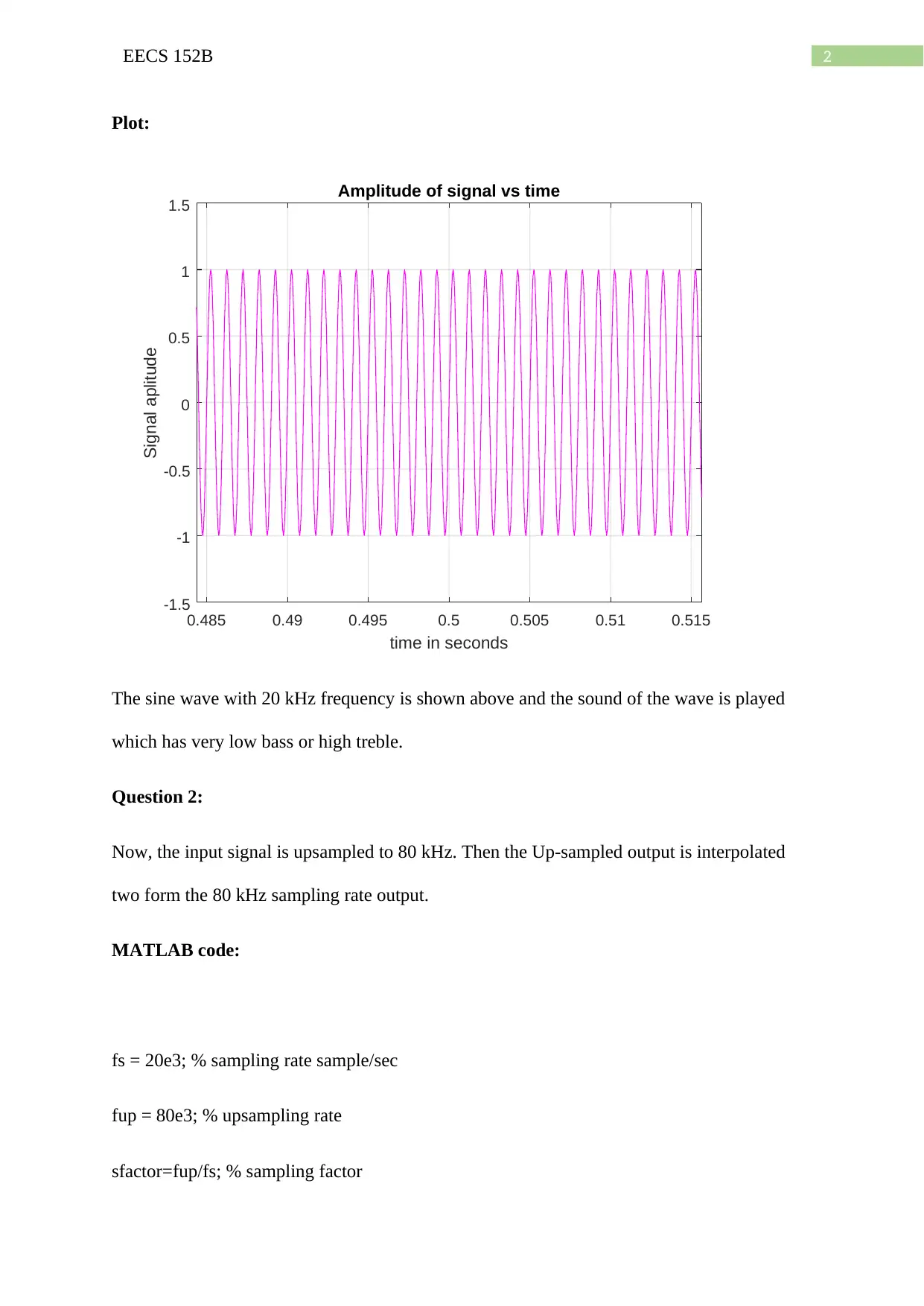
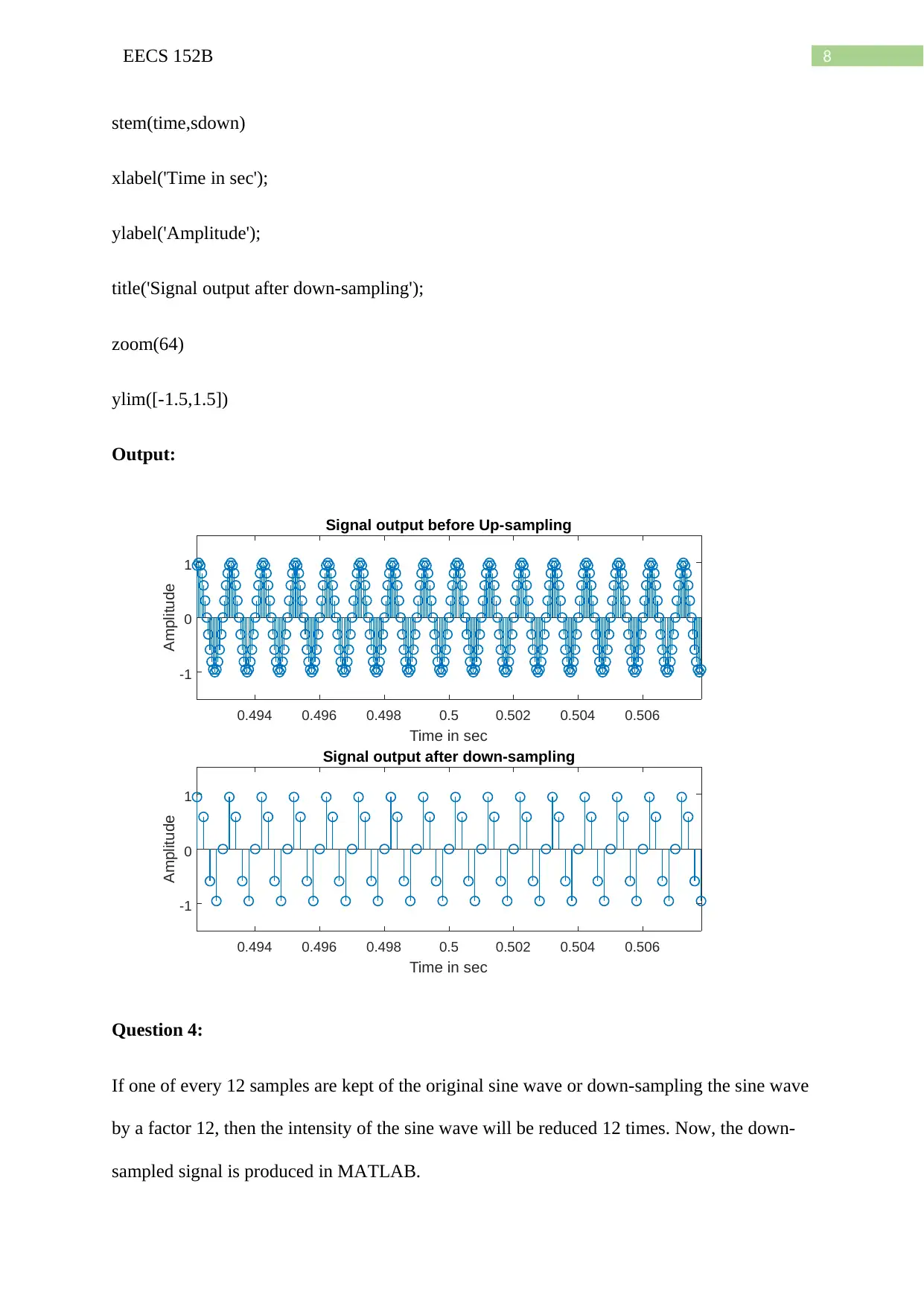
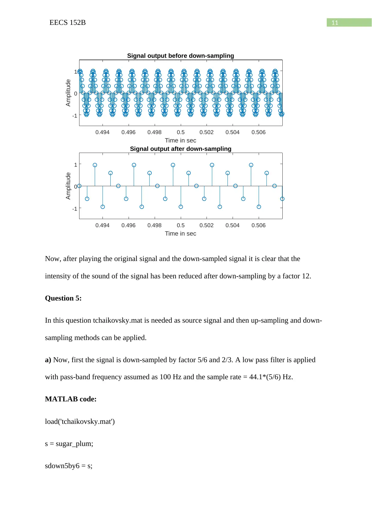
This assignment solution for EECS 152B, focuses on sample rate conversion techniques using MATLAB. It begins by generating and analyzing a 1000 Hz sine wave sampled at 20 kHz, playing the sound, and observing the effect. The solution then addresses upsampling to 80 kHz, exploring zero insertion and interpolation, and comparing the sound before and after each process. Next, the assignment investigates downsampling to 5 kHz and the necessity of anti-aliasing filters to mitigate aliasing effects. Further, the solution examines downsampling by a factor of 12 and its impact on signal intensity. Finally, it uses the 'tchaikovsky.mat' file to explore downsampling with factors 5/6 and 2/3, applying low-pass filters, and then downsampling with factors 1/2, 1/3 and 1/6. The solution also covers upsampling with factors 3/2, 9/2, and 21/2, applying low-pass filters and linear interpolator filters to remove aliasing effects and comparing the outcomes. The assignment demonstrates the effects of different rate conversion techniques on signal quality and the importance of filtering.

Running head: EECS 152B
EECS 152B
Name of the Student
Name of the University
Author Note

1EECS 152B
Question 1:
The MATLAB code for generating samples of a sin wave having frequency 1000 Hz which is
sampled by rate 20 kHz is given below. Then the sound command is used to listen the signal
as sound wave.
MATLAB code:
fs = 20e3; % sampling rate sample/sec
delt = 1/fs; % time increment sec/sample
t = 0:delt:1;
f = 1e3; % frequency of signal
s = sin(2*pi*f*t); % signal amplitude is 1
plot(t,s,'m')
xlabel('time in seconds');
ylabel('Signal aplitude');
title('Amplitude of signal vs time')
grid on
zoom(32)
ylim([-1.5,1.5])
sound(s,fs)

2EECS 152B
Plot:
0.485 0.49 0.495 0.5 0.505 0.51 0.515
time in seconds
-1.5
-1
-0.5
0
0.5
1
1.5
Signal aplitude
Amplitude of signal vs time
The sine wave with 20 kHz frequency is shown above and the sound of the wave is played
which has very low bass or high treble.
Question 2:
Now, the input signal is upsampled to 80 kHz. Then the Up-sampled output is interpolated
two form the 80 kHz sampling rate output.
MATLAB code:
fs = 20e3; % sampling rate sample/sec
fup = 80e3; % upsampling rate
sfactor=fup/fs; % sampling factor

3EECS 152B
delt = 1/fs; % time increment sec/sample
t = 0:delt:1;
f = 1e3; % frequency of signal
s = sin(2*pi*f*t); % signal amplitude is 1
figure(1)
subplot(2,1,1)
stem(t,s)
xlabel('Time in sec');
ylabel('Amplitude');
title('Signal output before Up-sampling');
zoom(64)
ylim([-1.5,1.5])
%%% zero insertion
lx = length(s);
y = 0;
y(1) = s(1);
for i=2:lx
c = [zeros(1,sfactor-1),s(i)];
y = [y,c];

4EECS 152B
end
%%% Output display of zeros inserted signal
nm=linspace(0,1,length(y));
figure(1)
subplot(2,1,2)
stem(nm,y); %Upsampled version of signal
xlabel('Time in sec');
ylabel('Amplitude');
title('Zeros inserted Output of Signal');
zoom(64)
ylim([-1.5,1.5])
sound(y,fup)
xi=s;
yi = interp(xi,sfactor);
nn=linspace(0,1,length(yi));
figure(2)
stem(nn,yi); %interpolation output
xlabel('Time in sec');
ylabel('Amplitude');

5EECS 152B
title('Up-sampled output after interpolation');
zoom(64)
ylim([-1.5,1.5])
sound(yi,fup)
Plots:

6EECS 152B
Now, it can be seen that the signal after inserting zeroes in between the intensity of sound
lessens. However, after interpolating the intensity of the sound was improved more than the
20 kHz sampled signal.
Question 3:
Now, the original signal is down-sampled to 5 kHz from 20 kHz keeping the frequency of the
signal same. If the signal is down-sampled then distortion happens due to aliasing. Now, to
nullify the aliasing effect anti-aliasing filters are applied. Now, the MATLAB code without
application of anti-aliasing filter is shown below.
MATLAB code:
fs = 20e3; % sampling rate sample/sec
fdown = 5e3; % upsampling rate

7EECS 152B
sfactor=fs/fdown; % down-sampling factor
delt = 1/fs; % time increment sec/sample
t = 0:delt:1;
f = 1e3; % frequency of signal
s = sin(2*pi*f*t); % signal amplitude is 1
figure(1)
subplot(2,1,1)
stem(t,s)
xlabel('Time in sec');
ylabel('Amplitude');
title('Signal output before Up-sampling');
zoom(64)
ylim([-1.5,1.5])
sdown = [];
for i=1:sfactor:length(s)
sdown = [sdown s(i)];
end
time = linspace(0,1,length(sdown));
figure(1)
subplot(2,1,2)

8EECS 152B
stem(time,sdown)
xlabel('Time in sec');
ylabel('Amplitude');
title('Signal output after down-sampling');
zoom(64)
ylim([-1.5,1.5])
Output:
-1
0
1
Amplitude
Signal output before Up-sampling
0.494 0.496 0.498 0.5 0.502 0.504 0.506
Time in sec
-1
0
1
Amplitude
Signal output after down-sampling
0.494 0.496 0.498 0.5 0.502 0.504 0.506
Time in sec
Question 4:
If one of every 12 samples are kept of the original sine wave or down-sampling the sine wave
by a factor 12, then the intensity of the sine wave will be reduced 12 times. Now, the down-
sampled signal is produced in MATLAB.

9EECS 152B
MATLAB function:
fs = 20e3; % sampling rate sample/sec
sfactor=12; % down-sampling factor
fdown = fs/12; % down-sampled rate
delt = 1/fs; % time increment sec/sample
t = 0:delt:1;
f = 1e3; % frequency of signal
s = sin(2*pi*f*t); % signal amplitude is 1
sound(s,fs)
figure(1)
subplot(2,1,1)
stem(t,s)
xlabel('Time in sec');
ylabel('Amplitude');
title('Signal output before Up-sampling');
zoom(64)
ylim([-1.5,1.5])
sdown = [];
for i=1:sfactor:length(s)
sdown = [sdown s(i)];

10EECS 152B
end
time = linspace(0,1,length(sdown));
figure(1)
subplot(2,1,2)
stem(time,sdown)
xlabel('Time in sec');
ylabel('Amplitude');
title('Signal output after down-sampling');
zoom(64)
ylim([-1.5,1.5])
sound(sdown,fdown)
Plot:

11EECS 152B
-1
0
1
Amplitude
Signal output before down-sampling
0.494 0.496 0.498 0.5 0.502 0.504 0.506
Time in sec
-1
0
1
Amplitude
Signal output after down-sampling
0.494 0.496 0.498 0.5 0.502 0.504 0.506
Time in sec
Now, after playing the original signal and the down-sampled signal it is clear that the
intensity of the sound of the signal has been reduced after down-sampling by a factor 12.
Question 5:
In this question tchaikovsky.mat is needed as source signal and then up-sampling and down-
sampling methods can be applied.
a) Now, first the signal is down-sampled by factor 5/6 and 2/3. A low pass filter is applied
with pass-band frequency assumed as 100 Hz and the sample rate = 44.1*(5/6) Hz.
MATLAB code:
load('tchaikovsky.mat')
s = sugar_plum;
sdown5by6 = s;

12EECS 152B
sdown2by3 = s;
fs = 44.1e3;
t = linspace(0,1,length(s));
figure(1)
subplot(2,1,1)
plot(t,s)
xlabel('Time in sec');
ylabel('Amplitude');
title('Original Signal output');
zoom(64)
ylim([-0.03,0.03])
%%% down-sampling by factor 5/6.
n=1;i=6*n;
while i<=length(s)
while i<=length(s)
sdown5by6(i) = 0; %% every 6n element in the signal is made equal to zero. 6n less than
signal length
i=6*n;
n=n+1;

13EECS 152B
end
end
sdown5by6 = nonzeros(sdown5by6); %% removing zero points from the signal
%%%applying low-pass filter
sdown5by6 = lowpass(sdown5by6,100,fs*(5/6)); %% passband frequency is assumed to be
100 Hz
t1 = linspace(0,1,length(sdown5by6));
figure(1)
subplot(2,1,2)
plot(t1,sdown5by6)
xlabel('Time in sec');
ylabel('Amplitude');
title('Dowsampled Signal by factor 5/6');
zoom(64)
ylim([-0.03,0.03])
%%% down-sampling by factor 2/3
n=1;i=3*n;

14EECS 152B
while i<=length(s)
while i<=length(s)
sdown2by3(i) = 0; %% every 3n element in the signal is made equal to zero. 3n less than
signal length
i=3*n;
n=n+1;
end
end
sdown2by3 = nonzeros(sdown2by3); %% removing zero points from the signal
sdown2by3 = lowpass(sdown2by3,100,fs*(2/3)); %% passband frequency is assumed to be
100 Hz
t2 = linspace(0,1,length(sdown2by3));
figure(2)
subplot(2,1,1)
plot(t,s)
xlabel('Time in sec');
ylabel('Amplitude');
title('Original Signal output');
zoom(64)
ylim([-0.03,0.03])

15EECS 152B
subplot(2,1,2)
plot(t2,sdown2by3)
xlabel('Time in sec');
ylabel('Amplitude');
title('Dowsampled Signal by factor 2/3');
zoom(64)
ylim([-0.03,0.03])
Plot:
0.494 0.496 0.498 0.5 0.502 0.504 0.506
Time in sec
-0.02
0
0.02
Amplitude
Original Signal output
0.494 0.496 0.498 0.5 0.502 0.504 0.506
Time in sec
-0.02
0
0.02
Amplitude
Dowsampled Signal by factor 5/6

16EECS 152B
0.494 0.496 0.498 0.5 0.502 0.504 0.506
Time in sec
-0.02
0
0.02
Amplitude
Original Signal output
0.494 0.496 0.498 0.5 0.502 0.504 0.506
Time in sec
-0.02
0
0.02
Amplitude
Dowsampled Signal by factor 2/3
Now, down-sampling is done on the signal and no low pass filters are applied. The signal is
down-sampled by factors ½, 1/3 and 1/6 respectively.
MATLAB code:
load('tchaikovsky.mat')
s = sugar_plum;
fs = 44.1e3;
t = linspace(0,1,length(s));
sdown1by2 = s;
%%% down-sampling by factor 1/2.
n=1;i=2*n;
while i<=length(s)

17EECS 152B
while i<=length(s)
sdown1by2(i) = 0; %% every 6n element in the signal is made equal to zero. 6n less than
signal length
i=2*n;
n=n+1;
end
end
sdown1by2 = nonzeros(sdown1by2); %% removing zero points from the signal
t1 = linspace(0,1,length(sdown1by2));
figure(1)
subplot(2,1,1)
plot(t,s)
xlabel('Time in sec');
ylabel('Amplitude');
title('Original Signal output');
subplot(2,1,2)
plot(t1,sdown1by2)
xlabel('Time in sec');
ylabel('Amplitude');
title('Downsampled Signal by factor 1/2');

18EECS 152B
zoom(64)
ylim([-0.03,0.03])
%sound(sdown1by2)
%%% down-sampling by factor 1/3.
sfactor=3;
sdown1by3 = downsample(s,sfactor);
t1 = linspace(0,1,length(sdown1by3));
figure(2)
subplot(2,1,1)
plot(t,s)
xlabel('Time in sec');
ylabel('Amplitude');
title('Original Signal output');
subplot(2,1,2)
plot(t1,sdown1by3)
xlabel('Time in sec');

19EECS 152B
ylabel('Amplitude');
title('Dowsampled Signal by factor 1/3');
zoom(64)
ylim([-0.03,0.03])
%sound(sdown1by3)
%%% down-sample by factor 1/6
sfactor=6;
sdown1by6 = downsample(s,sfactor);
t1 = linspace(0,1,length(sdown1by6));
figure(3)
subplot(2,1,1)
plot(t,s)
xlabel('Time in sec');
ylabel('Amplitude');
title('Original Signal output');
subplot(2,1,2)
plot(t1,sdown1by6)

20EECS 152B
xlabel('Time in sec');
ylabel('Amplitude');
title('Dowsampled Signal by factor 1/6');
zoom(64)
ylim([-0.03,0.03])
sound(sdown1by6)
Plot:
0 0.1 0.2 0.3 0.4 0.5 0.6 0.7 0.8 0.9 1
Time in sec
-0.2
-0.1
0
0.1
0.2
Amplitude
Original Signal output
0.494 0.496 0.498 0.5 0.502 0.504 0.506
Time in sec
-0.02
0
0.02
Amplitude
Downsampled Signal by factor 1/2

21EECS 152B
0 0.1 0.2 0.3 0.4 0.5 0.6 0.7 0.8 0.9 1
Time in sec
-0.2
-0.1
0
0.1
0.2
Amplitude
Original Signal output
0.494 0.496 0.498 0.5 0.502 0.504 0.506
Time in sec
-0.02
0
0.02
Amplitude
Dowsampled Signal by factor 1/3
0 0.1 0.2 0.3 0.4 0.5 0.6 0.7 0.8 0.9 1
Time in sec
-0.2
-0.1
0
0.1
0.2
Amplitude
Original Signal output
0.494 0.496 0.498 0.5 0.502 0.504 0.506
Time in sec
-0.02
0
0.02
Amplitude
Dowsampled Signal by factor 1/6

22EECS 152B
Now, it is evident that when the low pass filter is applied after down-sampling the sound
quality is do not affected much as aliasing effect is reduced. However, in the raw down-
sampled output of signal have aliasing and thus the quality is less.
b)
Now, the signal is up-sampled by factors 3/2, 9/2 and 21/2. This is done by first up-sampling
the signal and then down-sampling the up-sampled signal. Like for up-sampling by factor 3/2
the signal is first up-sampled by factor 3 and it is down-sampled by factor 2. After, that a low
pass filter with pass band frequency 100 Hz and sampling rate of (44.1)*(up sampling factor)
kHz is applied to the signal to remove aliasing effect. The same is done for all up-sampling
factor process.
MATLAB code:
load('tchaikovsky.mat')
fs = 44.1e3;
s = nonzeros(sugar_plum);
%up sampling by factor 3/2
sup3by2 = downsample(upsample(s,3),2);
%%% applying low pass anti-alliasing filter
sup3by2filtered = lowpass(sup3by2,100,fs*(3/2));
t = linspace(0,1,length(sup3by2filtered));
figure(1)
subplot(2,2,1)

23EECS 152B
plot(t,sup3by2filtered)
xlabel('Time in sec');
ylabel('Amplitude');
title('Upsampled by factor 3/2');
%up sampling by factor 9/2
sup9by2 = downsample(upsample(s,9),2);
%%% applying low pass anti-alliasing filter
sup9by2filtered = lowpass(sup9by2,100,fs*(9/2));
t = linspace(0,1,length(sup9by2filtered));
figure(1)
subplot(2,2,2)
plot(t,sup9by2filtered)
xlabel('Time in sec');
ylabel('Amplitude');
title('Upsampled by factor 9/2');
%up sampling by factor 21/2
sup21by2 = downsample(upsample(s,21),2);
%%% applying low pass anti-alliasing filter

24EECS 152B
sup21by2filtered = lowpass(sup21by2,100,fs*(21/2));
t = linspace(0,1,length(sup21by2filtered));
figure(1)
subplot(2,2,[3,4])
plot(t,sup21by2filtered)
xlabel('Time in sec');
ylabel('Amplitude');
title('Upsampled by factor 21/2');
Plot:
0 0.5 1
Time in sec
-0.05
0
0.05
Amplitude
Upsampled by factor 3/2
0 0.5 1
Time in sec
-0.02
-0.01
0
0.01
0.02
Amplitude
Upsampled by factor 9/2
0 0.1 0.2 0.3 0.4 0.5 0.6 0.7 0.8 0.9 1
Time in sec
-0.01
-0.005
0
0.005
0.01
Amplitude
Upsampled by factor 21/2

25EECS 152B
c) Now, in this task the anti-aliasing filter after resampling is chosen to be a linear
interpolator filter instead of a low pass filter. This filter is applied in all the up-sampling
factor process.
MATLAB code:
load('tchaikovsky.mat')
fs = 44.1e3;
s = nonzeros(sugar_plum);
%up sampling by factor 3/2
sup3by2 = downsample(upsample(s,3),2);
%%% applying linear interpolar filter
t = linspace(0,1,length(s));
tq = linspace(0,1,length(sup3by2));
sup3by2filtered = interp1(t,s,tq,'linear');
figure(1)
subplot(2,2,1)
plot(tq,sup3by2filtered)
xlabel('Time in sec');
ylabel('Amplitude');
title('Upsampled by factor 3/2 with linear interpolator filter');

26EECS 152B
%up sampling by factor 9/2
sup9by2 = downsample(upsample(s,9),2);
%%% applying low pass anti-alliasing filter
tq = linspace(0,1,length(sup9by2));
sup9by2filtered = interp1(t,s,tq,'linear');
figure(1)
subplot(2,2,2)
plot(tq,sup9by2filtered)
xlabel('Time in sec');
ylabel('Amplitude');
title('Upsampled by factor 9/2 with linear interpolator filter');
%up sampling by factor 21/2
sup21by2 = downsample(upsample(s,21),2);
%%% applying low pass anti-alliasing filter
tq = linspace(0,1,length(sup21by2));
sup21by2filtered = interp1(t,s,tq,'linear');
figure(1)

27EECS 152B
subplot(2,2,[3,4])
plot(tq,sup21by2filtered)
xlabel('Time in sec');
ylabel('Amplitude');
title('Upsampled by factor 21/2 with linear interpolator filter');
Plot:
0 0.1 0.2 0.3 0.4 0.5 0.6 0.7 0.8 0.9 1
Time in sec
-0.2
-0.15
-0.1
-0.05
0
0.05
0.1
0.15
Amplitude
Upsampled by factor 3/2 with linear interpolator filter
0 0.1 0.2 0.3 0.4 0.5 0.6 0.7 0.8 0.9 1
Time in sec
-0.2
-0.15
-0.1
-0.05
0
0.05
0.1
0.15
Amplitude
Upsampled by factor 9/2 with linear interpolator filter
0 0.1 0.2 0.3 0.4 0.5 0.6 0.7 0.8 0.9 1
Time in sec
-0.2
-0.15
-0.1
-0.05
0
0.05
0.1
0.15
Amplitude
Upsampled by factor 21/2 with linear interpolator filter
Now, by using linear interpolator filter rather than the low pass filter, the main advantage is
in low pass the all the high band frequencies over pass band will be eliminated but the
aliasing is not entirely removed, however in case of linear interpolator the in between points
after resampling are replaced by average values of the surrounding and hence the aliasing is
nullified by a greater extent.

28EECS 152B

29EECS 152B