EGB211 Computer Lab Assignment: Dynamics & Pendulum System Analysis

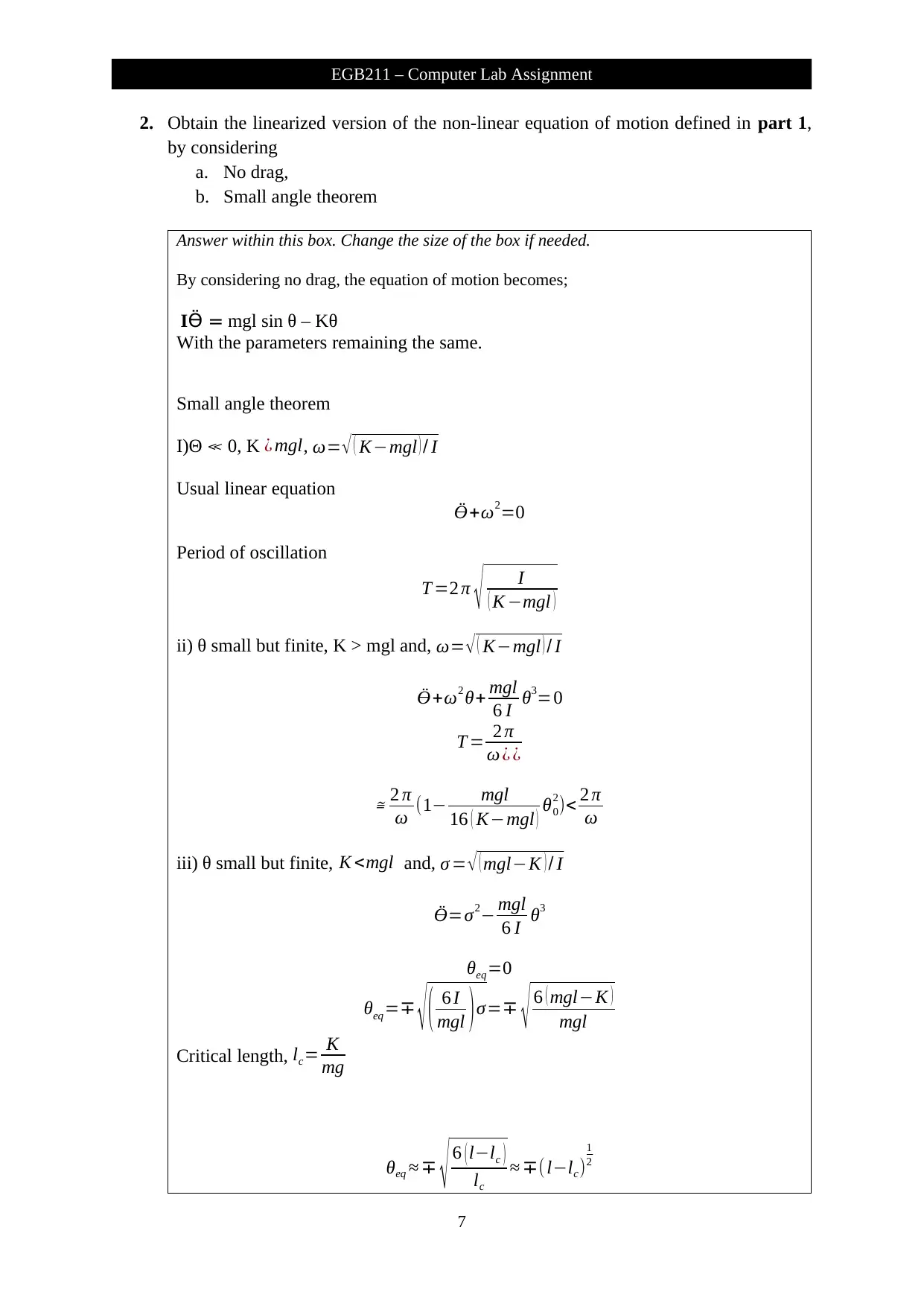
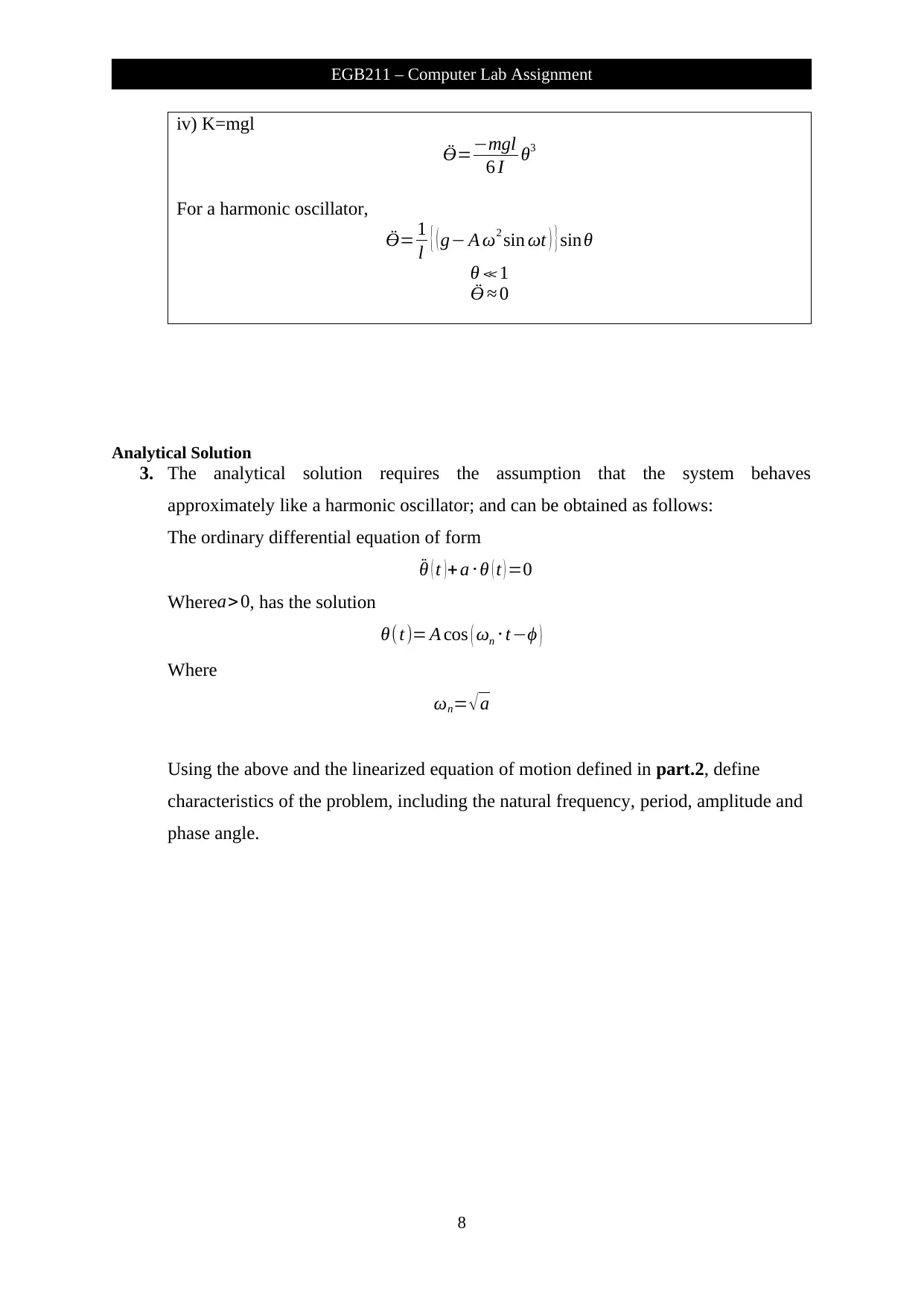
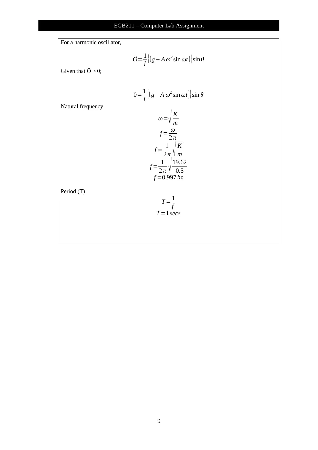
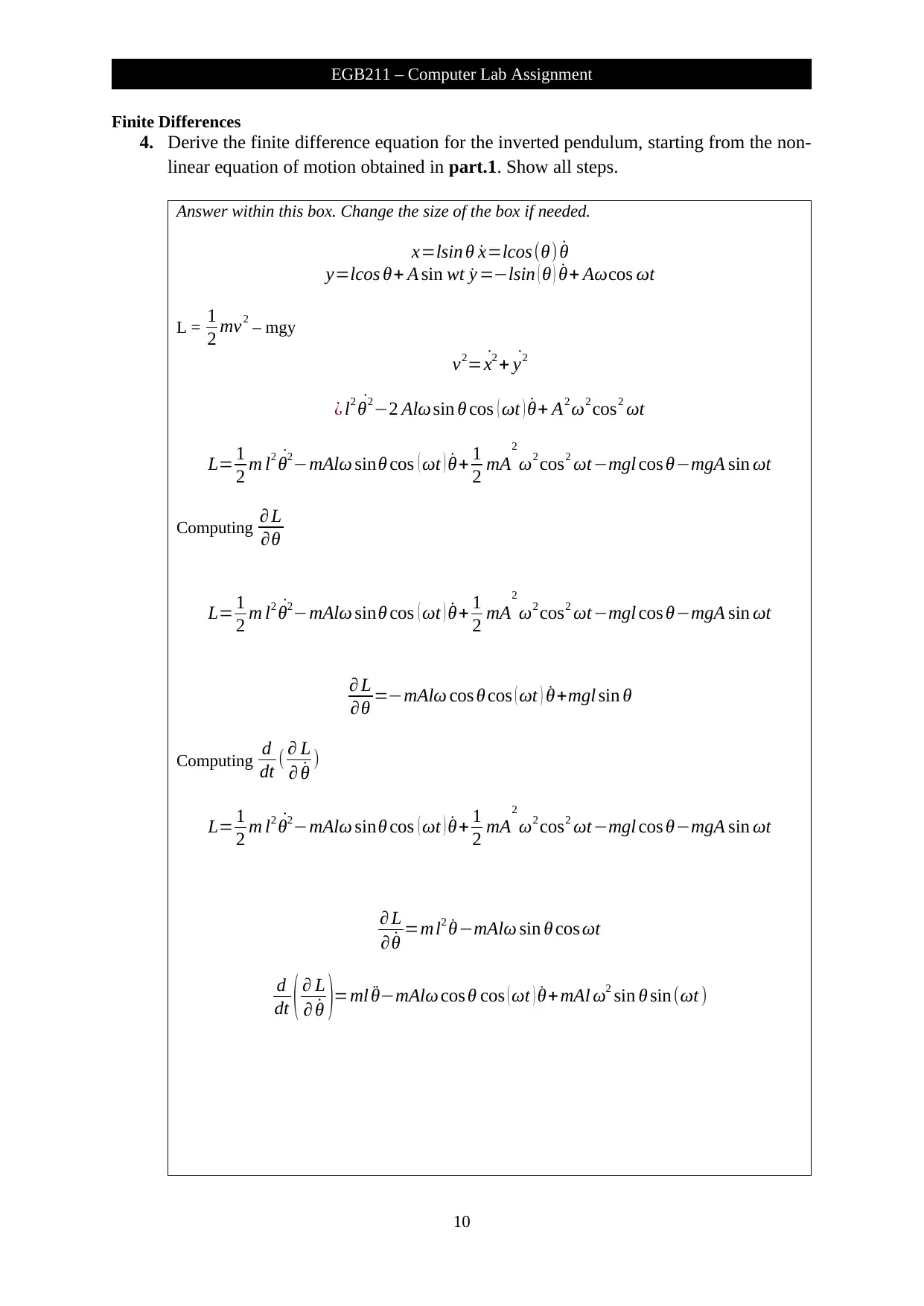
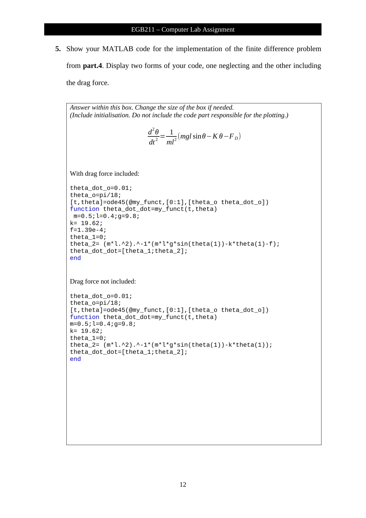
This EGB211 computer lab assignment delves into the dynamics of an inverted pendulum system, comparing analytical and numerical solutions. The assignment begins by deriving the equation of motion for the system, considering factors like gravity, spring force, and drag. It then linearizes the equation using the small angle theorem and develops an analytical solution based on harmonic oscillator principles. The assignment further explores numerical solutions using the finite difference method implemented in MATLAB, with and without considering drag force. The impact of the time-step on the accuracy of the numerical solution is analyzed, and the results from the analytical and numerical methods are compared graphically for angle, angular speed and angular acceleration. The MATLAB code for implementing the finite difference method is also provided. This comprehensive analysis provides insights into the behavior of non-linear dynamic systems and the application of numerical methods in solving complex engineering problems. Desklib provides a variety of assignment solutions and study tools for students.

1
EGB211 – Computer Lab Assignment
Assessment No: 3
Assessment Type: Individual Computer Lab Assignment
Due Date: Monday, 21st May 2018
Student ID:
Name:

EGB211 – Computer Lab Assignment
Dynamics is the subdivision of applied arithmetic (precisely classical mechanics) that deals
with the learning of forces and torques and their impact on motion. The learning of dynamics
falls further down to two groups: linear and rotational. Linear dynamics apply to bodies
moving in a line and encompasses such capacities as force, mass/inertia, displacement (in
units of distance), velocity , acceleration and momentum . Rotational dynamics apply to
bodies that are in rotary or moving in a curved track and comprises such capacities
as torque, moment of inertia/gyratory inertia, angular movement (in radians or less
repeatedly, degrees), angular velocity (radians per unit time), angular deceleration (radians
per unit of time squared) and angular motion (moment of inertia times unit of angular speed).
Over and over again, bodies display both linear and rotational motion (Goodman & Warner,
2013).
A dynamic problem can be divided in two phases: attaining the equation of motion and
answering it. In order to attain the equation of motion we use corporate dynamics concept,
such as Newton’s second law. The equation of motion can then be solved via analytical or
numerical methods. So far, you have frequently considered the analytical explanations to
problems, on the other hand even for simple dynamics problems these can promptly turn into
complex and unwieldy (think drag acting on a projectile). In the real world, the occurrence of
a true analytical solution is rare in many cases, and we rather rely on simplifications and
assumptions (e.g. neglecting drag). Numerical solutions on the other hand can be readily
used to solve simple and complex dynamics problems, without simplification (Forrester,
2013). In numerical solutions the main challenges become computational resources and the
elegance of the model.
In this computer lab assignment, we will explore the analytical and numerical solution to the
non-linear equation of motion of the inverted pendulum system illustrated in Figure. 1. For
small oscillations, we can apply the small angle theorem, linearizing the equation of motion,
allowing us to obtain an analytical solution. We will explore the impact of non-linearity and
the limits of linear assumption by comparison against the numerical solution for the non-
linear equation of motion. Finally, we explore the use of numerical methods as a tool to
investigate the real-world behaviour and characteristics of non-linear dynamics.
2
EGB211 – Computer Lab Assignment

Fig
ure 1. Diagram of the system (not to-scale)
Property Symbol Quantity Unit
Pendulum
Mass m 0.5 kg
Initial angle
with the vertical
axis (CCW)
ϑ 0 10 degrees
Initial angular
velocity ˙θ0 0.01 rad / s
Length l 0.4 m
Cross-sectional
area of mass A 0.05 m2
Spiral spring
constant k 19.62 Nm
rad
Drag
Air density ρ 1.183 kg /m3
Drag coefficient CD 0.47
Table 1. Quantities
For a dynamic analysis of the inverted pendulum system illustrated in Figure. 1 we will
consider the following.
 We will consider this as a one-dimensional problem in θ radians.
 The inverted pendulum rotates about O (x=0, y=0) and there is no restriction to the
rotation (i.e., number of full 360 ° turns).
 The spiral spring produces a moment kθ [ N ⋅m] at O.
 The bar connecting the spherical mass and spiral spring is assumed to be rigid and
have no mass.
 Unless situated in a complete vacuum, due to surrounding air drag force with a of
FD =−1
2 CD ρA v2 ⋅sign( v) is exerted on the spherical mass at the end of bar.
3
EGB211 – Computer Lab Assignment

Equation of Motion
1. Define the equation of motion for this inverted pendulum spring system in Figure 1.
Show all steps including a free-body-diagram (include drag).
Answer within this box. Change the size of the box if needed.
For a free body
m- mass of the body
torque = moment of inertia – angular acceleration
τnet = IӪ
Torque due to gravity
τnet = mgl sin θ
θ – angle in radians from the equilibrium position
Hence
IӪ = mgl sin θ
Moment of inertia
I = ml2
Therefore,
ml2Ӫ = mgl sin θ
after solving we obtain,
Ӫ = g
l sin θ
The equation above assumes no friction or any other resistance to movement.
The inverted pendulum in space is similar to the uninverted pendulum.
FD =−1
2 CD ρA v2 ⋅sign(v)
Equation for the inverted pendulum spring system
IӪ = mgl sin θ – Kθ - FD
K- elastic coefficient of the spiral spring
I – mass moment of inertia
m – weight of the translating mass
g – gravity
l – length
4
EGB211 – Computer Lab Assignment

K.E = 1
2 mv2
P.E = mgh
Lagrangian, L = K.E + P.E
Eulerlangrange equation d
dt ( ∂ L
∂ ˙θ )= ∂ L
∂ θ
Vertical motion, St = A sin ωt
L = 1
2 mv2 - mgh
V2 = ˙x2+ ˙y2
V2 = L2 ( ˙θ2 ) cos2 θ+ L2 ( ˙θ2 ) sin2 θ
= L2 ( ˙θ2 )
L = 1
2 m L2 ( ˙θ2 ) - mg l cos θ
d
dt ( ∂ L
∂ ˙θ )=ml2 Ӫ
∂ L
∂θ =mgl sin θ
Euler Lagrange
5
EGB211 – Computer Lab Assignment

d
dt ( ∂ L
∂ ˙θ )= ∂ L
∂ θ
ml2 Ӫ=mgl sinθ
Ӫ= g
l sin θ
Also, for a harmonic oscillator the equation of motion is given as;
Ӫ= 1
l { ( g− A ω2 sin ωt ) } sinθ
6
EGB211 – Computer Lab Assignment

2. Obtain the linearized version of the non-linear equation of motion defined in part 1,
by considering
a. No drag,
b. Small angle theorem
Answer within this box. Change the size of the box if needed.
By considering no drag, the equation of motion becomes;
I =Ӫ mgl sin θ – Kθ
With the parameters remaining the same.
Small angle theorem
I)Θ ≪ 0, K ¿ mgl, ω= √ ( K−mgl ) / I
Usual linear equation
Ӫ+ω2=0
Period of oscillation
T =2 π √ I
( K −mgl )
ii) θ small but finite, K > mgl and, ω= √ ( K−mgl ) / I
Ӫ+ω2 θ+ mgl
6 I θ3=0
T = 2 π
ω ¿ ¿
≅ 2 π
ω (1− mgl
16 ( K−mgl ) θ0
2)< 2 π
ω
iii) θ small but finite, K <mgl and, σ = √ ( mgl−K ) / I
Ӫ=σ2− mgl
6 I θ3
θeq=0
θeq=∓ √ ( 6 I
mgl )σ=∓ √ 6 ( mgl−K )
mgl
Critical length, lc= K
mg
θeq ≈ ∓ √ 6 ( l−lc )
lc
≈ ∓( l−lc)
1
2
7
EGB211 – Computer Lab Assignment

iv) K=mgl
Ӫ=−mgl
6 I θ3
For a harmonic oscillator,
Ӫ= 1
l { ( g− A ω2 sin ωt ) } sinθ
θ ≪ 1
Ӫ ≈ 0
Analytical Solution
3. The analytical solution requires the assumption that the system behaves
approximately like a harmonic oscillator; and can be obtained as follows:
The ordinary differential equation of form
¨θ ( t )+ a ⋅θ ( t ) =0
Wherea> 0, has the solution
θ(t)= A cos ( ωn ⋅t−ϕ )
Where
ωn= √ a
Using the above and the linearized equation of motion defined in part.2, define
characteristics of the problem, including the natural frequency, period, amplitude and
phase angle.
8
EGB211 – Computer Lab Assignment

For a harmonic oscillator,
Ӫ= 1
l { ( g− A ω2 sin ωt ) } sinθ
Given that Ӫ ≈ 0;
0=1
l { ( g−A ω2 sin ωt ) } sin θ
Natural frequency
ω= √ K
m
f = ω
2 π
f = 1
2 π √ K
m
f = 1
2 π √ 19.62
0.5
f =0.997 hz
Period (T)
T = 1
f
T =1 secs
9
EGB211 – Computer Lab Assignment

Finite Differences
4. Derive the finite difference equation for the inverted pendulum, starting from the non-
linear equation of motion obtained in part.1. Show all steps.
Answer within this box. Change the size of the box if needed.
x=lsin θ ˙x=lcos(θ) ˙θ
y=lcos θ+ A sin wt ˙y =−lsin ( θ ) ˙θ+ Aωcos ωt
L = 1
2 mv2 – mgy
v2= ˙x2 + ˙y2
¿ l2 ˙θ2−2 Alω sin θ cos ( ωt ) ˙θ+ A2 ω2 cos2 ωt
L= 1
2 m l2 ˙θ2−mAlω sinθ cos ( ωt ) ˙θ+ 1
2 mA
2
ω2 cos2 ωt−mgl cos θ−mgA sin ωt
Computing ∂ L
∂θ
L= 1
2 m l2 ˙θ2−mAlω sinθ cos ( ωt ) ˙θ+ 1
2 mA
2
ω2 cos2 ωt−mgl cos θ−mgA sin ωt
∂ L
∂θ =−mAlω cos θ cos ( ωt ) ˙θ+mgl sin θ
Computing d
dt ( ∂ L
∂ ˙θ )
L= 1
2 m l2 ˙θ2−mAlω sinθ cos ( ωt ) ˙θ+ 1
2 mA
2
ω2 cos2 ωt−mgl cos θ−mgA sin ωt
∂ L
∂ ˙θ =ml2 ˙θ−mAlω sin θ cos ωt
d
dt ( ∂ L
∂ ˙θ )=ml ¨θ−mAlω cos θ cos ( ωt ) ˙θ+ mAl ω2 sin θ sin (ωt )
10
EGB211 – Computer Lab Assignment

Solving by Euler LaGrange equation
d
dt ( ∂ L
∂ ˙θ )= ∂ L
∂ θ
ml ¨θ−mAlω cos θ cos ( ωt ) ˙θ+mAl ω2 sinθ sin ( ωt ) =¿ ¿
−mAlω cos θ cos ( ωt ) ˙θ+ mgl sin θ
l ¨θ− Al ω2 sin θ sin ( ωt )=¿ g sin θ ¿
d2 θ
dt2 = 1
l ¿
11
EGB211 – Computer Lab Assignment

5. Show your MATLAB code for the implementation of the finite difference problem
from part.4. Display two forms of your code, one neglecting and the other including
the drag force.
Answer within this box. Change the size of the box if needed.
(Include initialisation. Do not include the code part responsible for the plotting.)
d2 θ
dt2 = 1
ml2 (mgl sinθ−K θ−F D )
With drag force included:
theta_dot_o=0.01;
theta_o=pi/18;
[t,theta]=ode45(@my_funct,[0:1],[theta_o theta_dot_o])
function theta_dot_dot=my_funct(t,theta)
m=0.5;l=0.4;g=9.8;
k= 19.62;
f=1.39e-4;
theta_1=0;
theta_2= (m*l.^2).^-1*(m*l*g*sin(theta(1))-k*theta(1)-f);
theta_dot_dot=[theta_1;theta_2];
end
Drag force not included:
theta_dot_o=0.01;
theta_o=pi/18;
[t,theta]=ode45(@my_funct,[0:1],[theta_o theta_dot_o])
function theta_dot_dot=my_funct(t,theta)
m=0.5;l=0.4;g=9.8;
k= 19.62;
theta_1=0;
theta_2= (m*l.^2).^-1*(m*l*g*sin(theta(1))-k*theta(1));
theta_dot_dot=[theta_1;theta_2];
end
12
EGB211 – Computer Lab Assignment