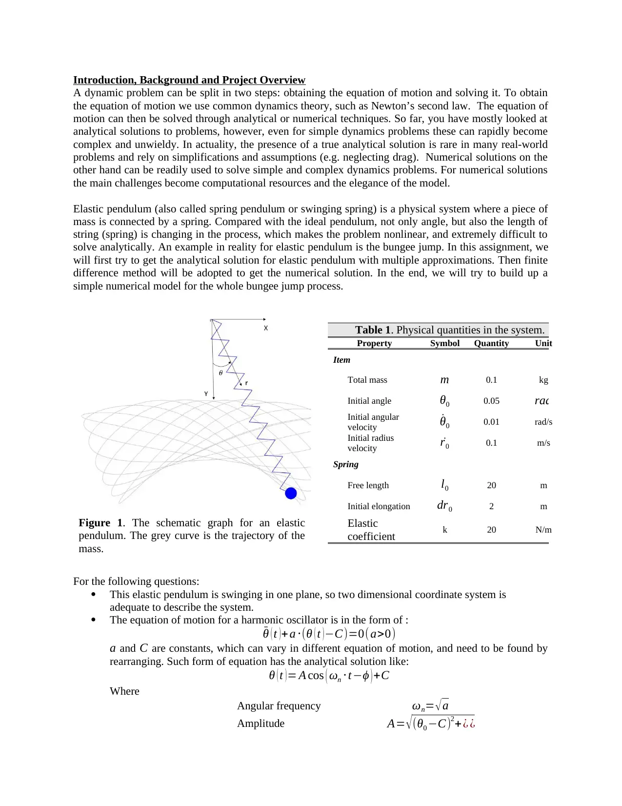
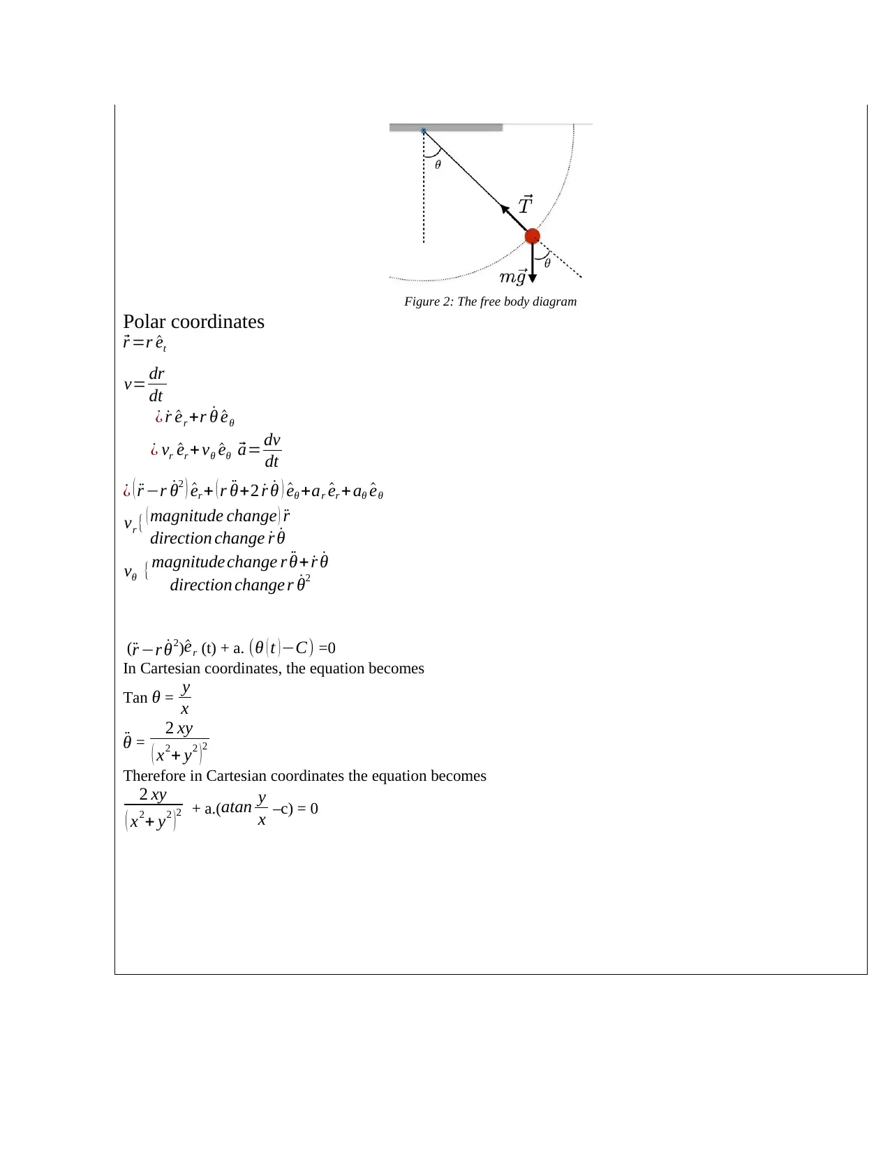
EGB211 Computer Lab Assignment 3: Analytical and Numerical Solutions

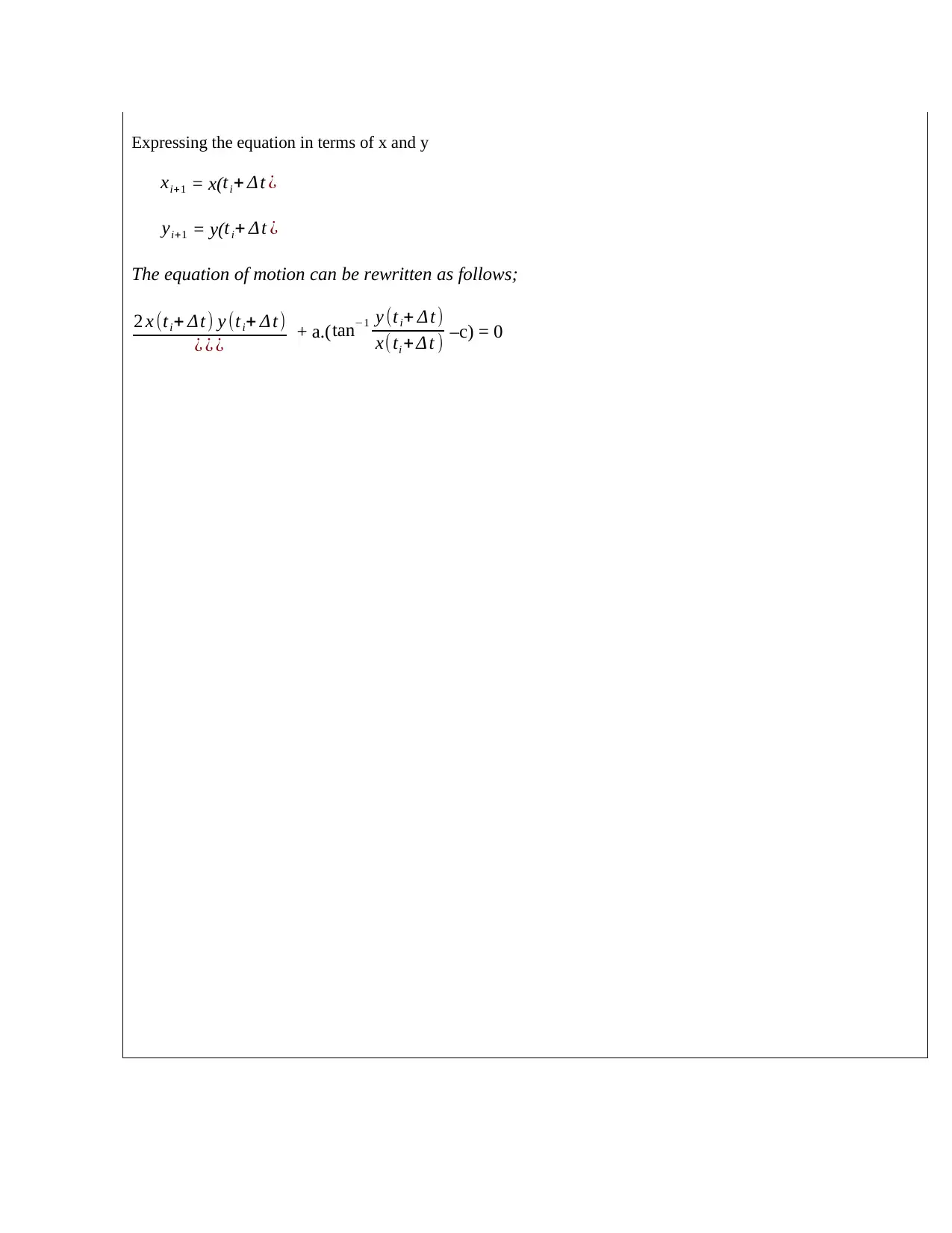
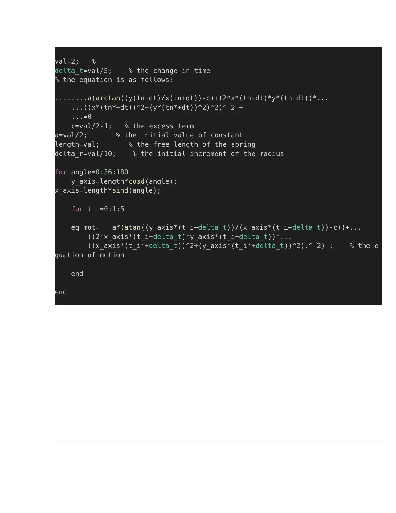
This assignment focuses on the analysis of an elastic pendulum, a dynamic system where a mass is connected to a spring. The assignment requires students to derive the equation of motion using both polar and Cartesian coordinate systems. It then explores analytical solutions using approximations and the finite difference method for numerical solutions. The assignment includes writing MATLAB code to solve the equations of motion and visualize the pendulum's trajectory. Students are tasked with comparing analytical and numerical solutions, exploring the impact of parameter changes, and developing a bungee jump simulation based on the elastic pendulum model. The assignment covers topics such as harmonic oscillation, discretization, convergence, and the application of numerical methods to real-world scenarios. The provided solution includes detailed derivations, MATLAB code, and analysis of the results.

Assessment No: 3
Assessment Type: Individual Computer Lab Assignment
Due Date: Friday, 11th October 2019
Student ID:
Name:

Introduction, Background and Project Overview
A dynamic problem can be split in two steps: obtaining the equation of motion and solving it. To obtain
the equation of motion we use common dynamics theory, such as Newton’s second law. The equation of
motion can then be solved through analytical or numerical techniques. So far, you have mostly looked at
analytical solutions to problems, however, even for simple dynamics problems these can rapidly become
complex and unwieldy. In actuality, the presence of a true analytical solution is rare in many real-world
problems and rely on simplifications and assumptions (e.g. neglecting drag). Numerical solutions on the
other hand can be readily used to solve simple and complex dynamics problems. For numerical solutions
the main challenges become computational resources and the elegance of the model.
Elastic pendulum (also called spring pendulum or swinging spring) is a physical system where a piece of
mass is connected by a spring. Compared with the ideal pendulum, not only angle, but also the length of
string (spring) is changing in the process, which makes the problem nonlinear, and extremely difficult to
solve analytically. An example in reality for elastic pendulum is the bungee jump. In this assignment, we
will first try to get the analytical solution for elastic pendulum with multiple approximations. Then finite
difference method will be adopted to get the numerical solution. In the end, we will try to build up a
simple numerical model for the whole bungee jump process.
Figure 1. The schematic graph for an elastic
pendulum. The grey curve is the trajectory of the
mass.
Table 1. Physical quantities in the system.
Property Symbol Quantity Unit
Item
Total mass m 0.1 kg
Initial angle θ0 0.05 rad
Initial angular
velocity ˙θ0 0.01 rad/s
Initial radius
velocity ˙r0 0.1 m/s
Spring
Free length l0 20 m
Initial elongation dr0 2 m
Elastic
coefficient k 20 N/m
For the following questions:
 This elastic pendulum is swinging in one plane, so two dimensional coordinate system is
adequate to describe the system.
 The equation of motion for a harmonic oscillator is in the form of :
¨θ ( t )+ a ⋅(θ ( t )−C)=0( a>0)
a and C are constants, which can vary in different equation of motion, and need to be found by
rearranging. Such form of equation has the analytical solution like:
θ ( t )= A cos ( ωn ⋅t−ϕ ) +C
Where
Angular frequency ωn= √ a
Amplitude A= √ (θ0 −C)2+¿ ¿

Phase ϕ =atan ¿
 Small angle theorem: when θ<5o , sinθ≈ θ, cosθ ≈ 1.

Equation of Motion
1. Draw the free body diagram for the elastic pendulum model in the Fig 1. Write down the
equations of motion in polar coordinate systems, and Cartesian coordinate system.
Answer within this box. Change the size of the box if needed.

Figure 2: The free body diagram
Polar coordinates ⃗
r =r ^et
v= dr
dt
¿ ˙r ^er +r ˙θ ^eθ
¿ vr ^er + vθ ^eθ ⃗ a= dv
dt
¿ ( ¨r −r ˙θ2 ) ^er + ( r ¨θ+2 ˙r ˙θ ) ^eθ +ar ^er + aθ ^eθ
vr { ( magnitude change ) ¨r
direction change ˙r ˙θ
vθ {magnitude change r ¨θ+ ˙r ˙θ
direction change r ˙θ2
(¨r −r ˙θ2) ^er (t) + a. (θ ( t )−C) =0
In Cartesian coordinates, the equation becomes
Tan θ = y
x
¨θ = 2 xy
( x2+ y2 ) 2
Therefore in Cartesian coordinates the equation becomes
2 xy
( x2+ y2 )2 + a.(atan y
x –c) = 0

Analytical Solution
2. To get the analytical solution, for a tough spring and a small mass, we can use the following
assumption:
 The elastic pendulum does harmonic oscillation in θ and r direction.
 In r direction, the oscillation of the spring is the dominate motion, and terms relevant with θ
can be ignored.
 In θ direction, the change of the spring length can be ignored, terms with r can be ignored.
Arrange the equation of motion in polar coordinate system to the harmonic oscillation form: (1)
use small angle theorem first, (2) then delete extra non-linear terms for approximation. Get the
analytical solution of elastic pendulum with the parameters in the table 1.
Answer within this box. Change the size of the box if needed.

⃗r =r ^et ,v= dr
dt
¿ ˙r ^er +r ˙θ ^eθ
¿ vr ^er + vθ ^eθ ⃗ a= dv
dt
¿ ( ¨r −r ˙θ2 ) ^er + ( r ¨θ+2 ˙r ˙θ ) ^eθ +ar ^er + aθ ^eθ
vr { ( magnitude change ) ¨r
direction change ˙r ˙θ
vθ {magnitude change r ¨θ+ ˙r ˙θ
direction change r ˙θ2
( ¨r −r ˙θ2) ^er (t) + a. (θ ( t ) −C) =0
θ ( t ) = A cos ( ωn ⋅t−ϕ ) …
Since it is known that A= √ (θ0 −C)2+ ¿ ¿, ωn= √ a and ϕ =atan ¿, the exact solution now becomes;
θ ( t )= √(θ0−C)2 +¿ ¿
replacing C with zero and Given that θ0 =0.005 and ˙θ0 = 0.1 rad/s
θ ( t )=¿
θ ( t )= √(0.05)2 +¿ ¿
∴
= ( √ 0.0025+ 0.01
a ) cos ( √ a⋅ t−atan ( 0.1
0.05∗√ a ))

Finite Differences
3. Write down the equation of motion in Cartesian coordinate system from Question 1 in the finite
difference form. State the initial conditions for finite difference method. Show all working.
Answer within this box. Change the size of the box if needed.

Expressing the equation in terms of x and y
xi+1 = x(ti+ Δt ¿
yi+1 = y( ti+ Δt ¿
The equation of motion can be rewritten as follows;
2 x (ti+ Δt ) y (ti+ Δt)
¿ ¿ ¿ + a.( tan−1 y (ti+ Δ t)
x(ti + Δt ) –c) = 0

MATLAB Code
4. Show the MATLAB code for solving the finite difference equations obtained in Question 3.
Answer within this box. Change the size of the box if needed.
(Include initialisation based on Question 3. Do not include the code part responsible for the plotting.)

val=2; %
delta_t=val/5; % the change in time
% the equation is as follows;
........a(arctan((y(tn+dt)/x(tn+dt))-c)+(2*x*(tn+dt)*y*(tn+dt))*...
...((x*(tn*+dt))^2+(y*(tn*+dt))^2)^2)^-2 +
...=0
c=val/2-1; % the excess term
a=val/2; % the initial value of constant
length=val; % the free length of the spring
delta_r=val/10; % the initial increment of the radius
for angle=0:36:180
y_axis=length*cosd(angle);
x_axis=length*sind(angle);
for t_i=0:1:5
eq_mot= a*(atan((y_axis*(t_i+delta_t))/(x_axis*(t_i+delta_t))-c))+...
((2*x_axis*(t_i+delta_t)*y_axis*(t_i+delta_t))*...
((x_axis*(t_i*+delta_t))^2+(y_axis*(t_i*+delta_t))^2).^-2) ; % the e
quation of motion
end
end

Discretization and Convergence:
5. The accuracy of numerical solution is completely dependent on the timestep dt. The accuracy and
the computational cost both increase indefinitely as dt → 0. Because of this, in practical
application of computational resources, we are only interested in dt which will provide results
that do not change/benefit from any further increase in resolution.
1) Estimate the dt value according to the frequency in Question 2. There should be at least 40
points in one period in each direction.
2) Plot the trajectory of the elastic pendulum from the numerical solution (x-y plot), with at least
2 periods in each direction.
Answer within this box. Change the size of the box if needed.