EGH418 Biomechanics: Beam Theory, Stress-Strain Curves & Data Analysis

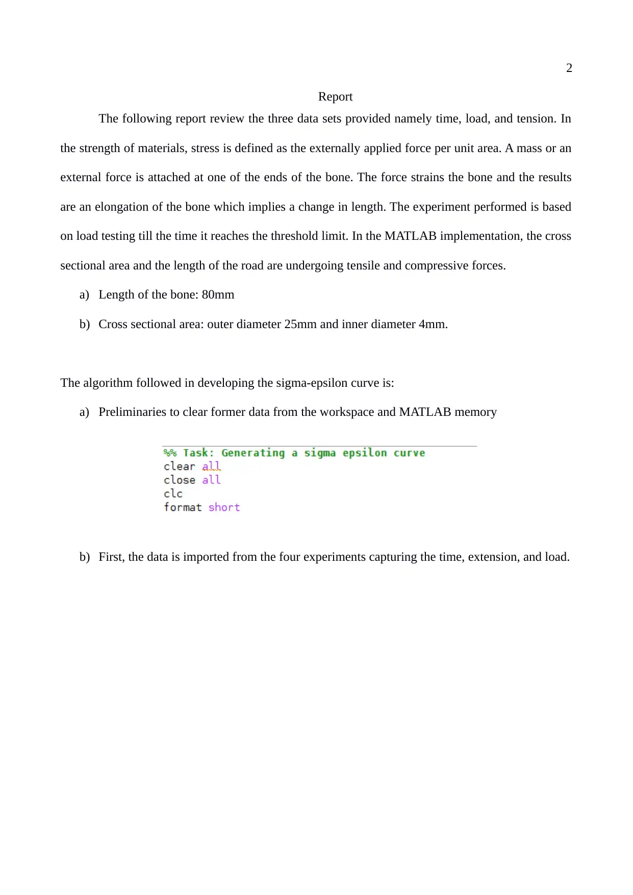
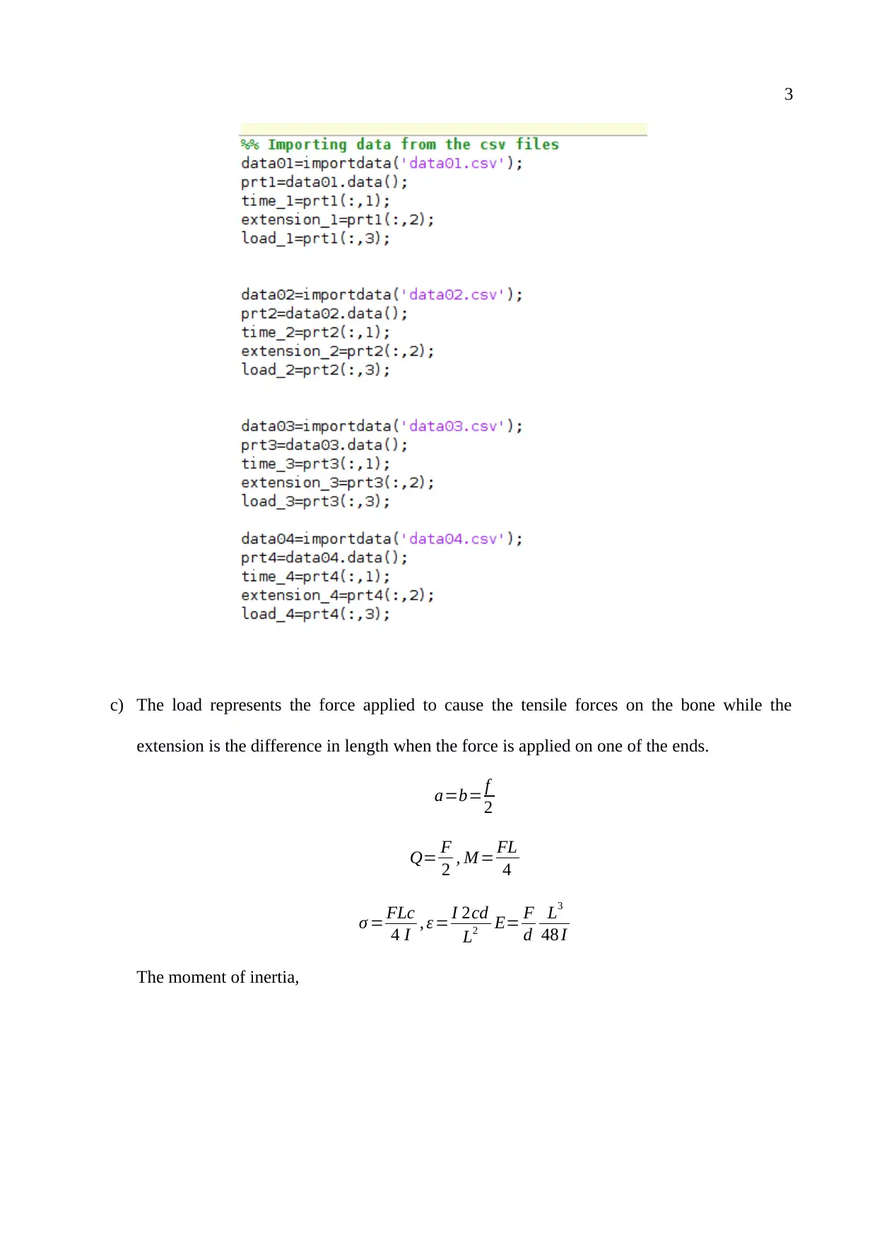
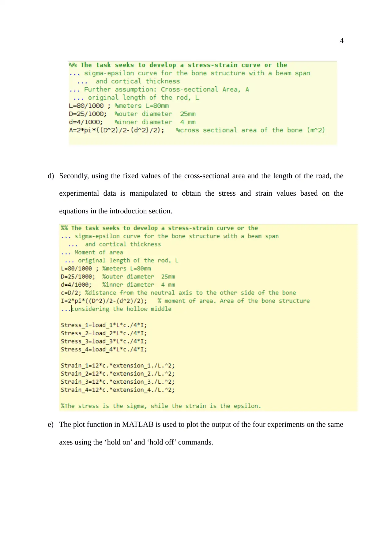
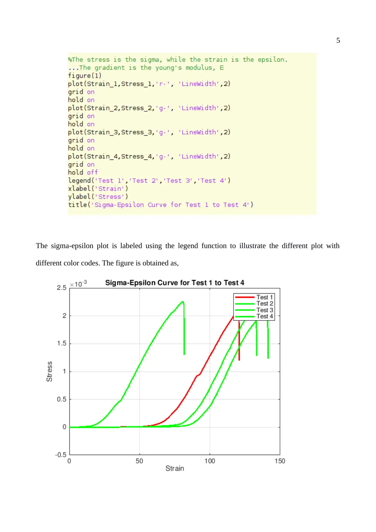
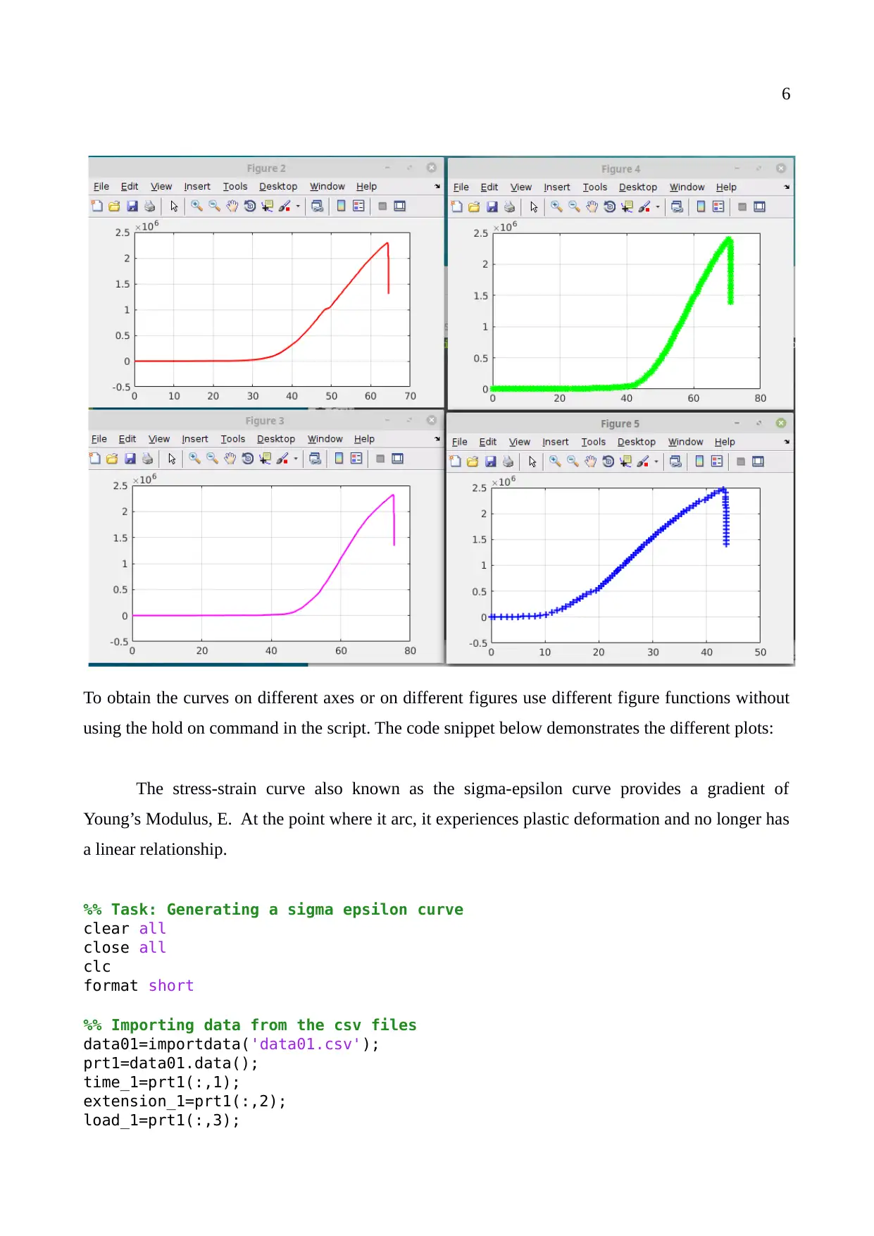
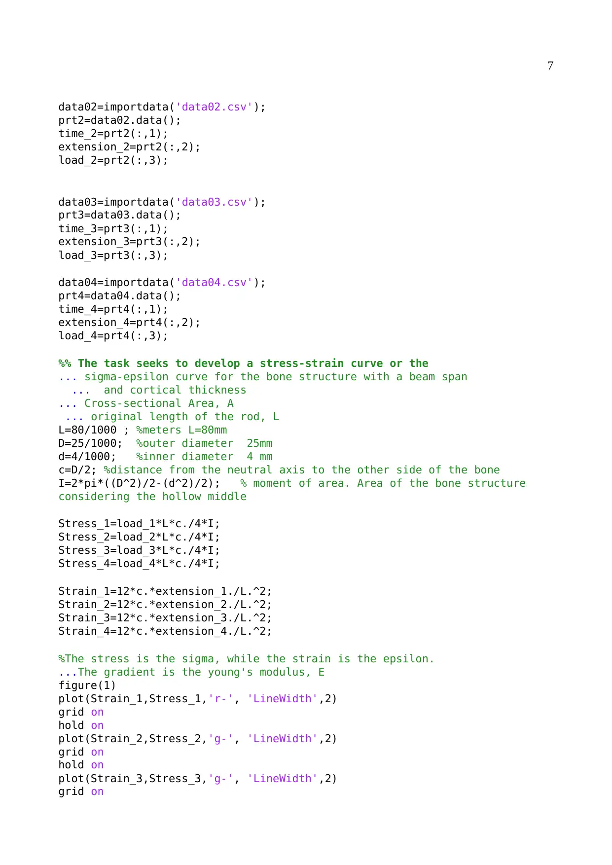
This report reviews three datasets (time, load, and tension) to analyze stress and strain in bone structures using beam theory. The experiment simulates load testing to a threshold limit, with MATLAB used to model tensile and compressive forces on a bone with specified dimensions. The algorithm imports data from four experiments, calculates stress and strain values based on the provided equations, and plots the sigma-epsilon curves for each experiment. The resulting plots illustrate the material's behavior under stress, including Young's Modulus, and identify the point of plastic deformation. The MATLAB code snippet provided demonstrates the data import, calculation, and plotting process, differentiating each experiment using color codes and legends. Desklib provides students access to similar solved assignments and past papers.

1
EGH418 BIOMECHANICS
BEAM THEORY
Student Name
Student ID Number
Institutional Affiliation
Date of Submission

2
Report
The following report review the three data sets provided namely time, load, and tension. In
the strength of materials, stress is defined as the externally applied force per unit area. A mass or an
external force is attached at one of the ends of the bone. The force strains the bone and the results
are an elongation of the bone which implies a change in length. The experiment performed is based
on load testing till the time it reaches the threshold limit. In the MATLAB implementation, the cross
sectional area and the length of the road are undergoing tensile and compressive forces.
a) Length of the bone: 80mm
b) Cross sectional area: outer diameter 25mm and inner diameter 4mm.
The algorithm followed in developing the sigma-epsilon curve is:
a) Preliminaries to clear former data from the workspace and MATLAB memory
b) First, the data is imported from the four experiments capturing the time, extension, and load.

3
c) The load represents the force applied to cause the tensile forces on the bone while the
extension is the difference in length when the force is applied on one of the ends.
a=b= f
2
Q= F
2 , M = FL
4
σ = FLc
4 I , ε = I 2cd
L2 E= F
d
L3
48 I
The moment of inertia,

4
d) Secondly, using the fixed values of the cross-sectional area and the length of the road, the
experimental data is manipulated to obtain the stress and strain values based on the
equations in the introduction section.
e) The plot function in MATLAB is used to plot the output of the four experiments on the same
axes using the ‘hold on’ and ‘hold off’ commands.

5
The sigma-epsilon plot is labeled using the legend function to illustrate the different plot with
different color codes. The figure is obtained as,

6
To obtain the curves on different axes or on different figures use different figure functions without
using the hold on command in the script. The code snippet below demonstrates the different plots:
The stress-strain curve also known as the sigma-epsilon curve provides a gradient of
Young’s Modulus, E. At the point where it arc, it experiences plastic deformation and no longer has
a linear relationship.
%% Task: Generating a sigma epsilon curve
clear all
close all
clc
format short
%% Importing data from the csv files
data01=importdata('data01.csv');
prt1=data01.data();
time_1=prt1(:,1);
extension_1=prt1(:,2);
load_1=prt1(:,3);

7
data02=importdata('data02.csv');
prt2=data02.data();
time_2=prt2(:,1);
extension_2=prt2(:,2);
load_2=prt2(:,3);
data03=importdata('data03.csv');
prt3=data03.data();
time_3=prt3(:,1);
extension_3=prt3(:,2);
load_3=prt3(:,3);
data04=importdata('data04.csv');
prt4=data04.data();
time_4=prt4(:,1);
extension_4=prt4(:,2);
load_4=prt4(:,3);
%% The task seeks to develop a stress-strain curve or the
... sigma-epsilon curve for the bone structure with a beam span
... and cortical thickness
... Cross-sectional Area, A
... original length of the rod, L
L=80/1000 ; %meters L=80mm
D=25/1000; %outer diameter 25mm
d=4/1000; %inner diameter 4 mm
c=D/2; %distance from the neutral axis to the other side of the bone
I=2*pi*((D^2)/2-(d^2)/2); % moment of area. Area of the bone structure
considering the hollow middle
Stress_1=load_1*L*c./4*I;
Stress_2=load_2*L*c./4*I;
Stress_3=load_3*L*c./4*I;
Stress_4=load_4*L*c./4*I;
Strain_1=12*c.*extension_1./L.^2;
Strain_2=12*c.*extension_2./L.^2;
Strain_3=12*c.*extension_3./L.^2;
Strain_4=12*c.*extension_4./L.^2;
%The stress is the sigma, while the strain is the epsilon.
...The gradient is the young's modulus, E
figure(1)
plot(Strain_1,Stress_1,'r-', 'LineWidth',2)
grid on
hold on
plot(Strain_2,Stress_2,'g-', 'LineWidth',2)
grid on
hold on
plot(Strain_3,Stress_3,'g-', 'LineWidth',2)
grid on

8
hold on
plot(Strain_4,Stress_4,'g-', 'LineWidth',2)
grid on
hold off
legend('Test 1','Test 2','Test 3','Test 4')
xlabel('Strain')
ylabel('Stress')
title('Sigma-Epsilon Curve for Test 1 to Test 4')