ELE2704 Electrical Power: Short Transmission Line Performance

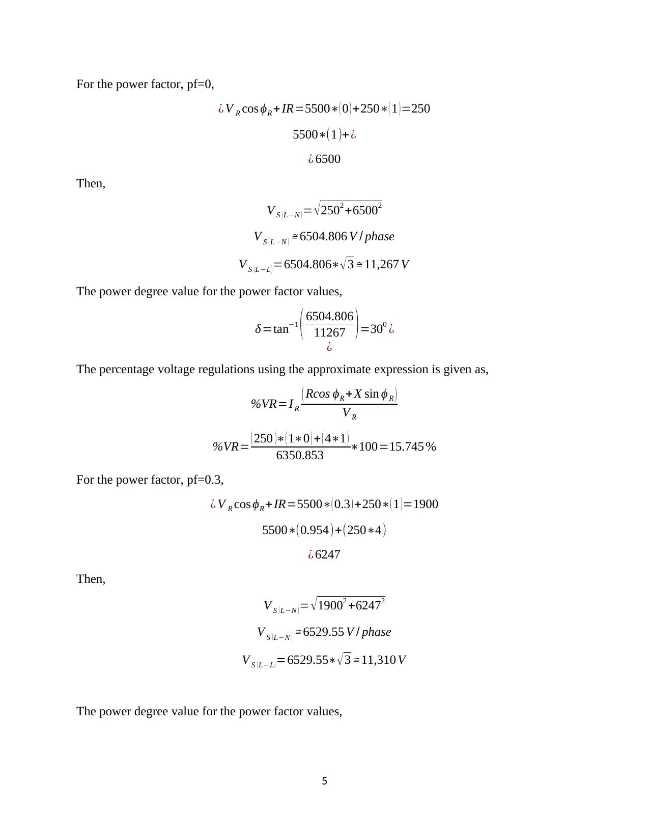
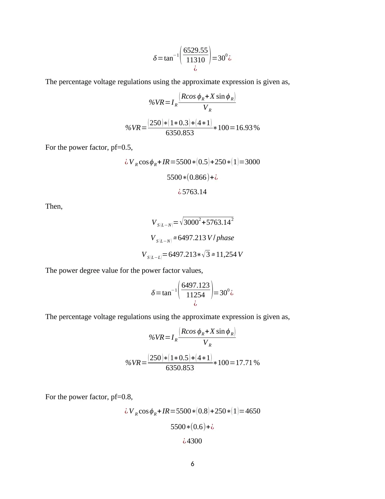
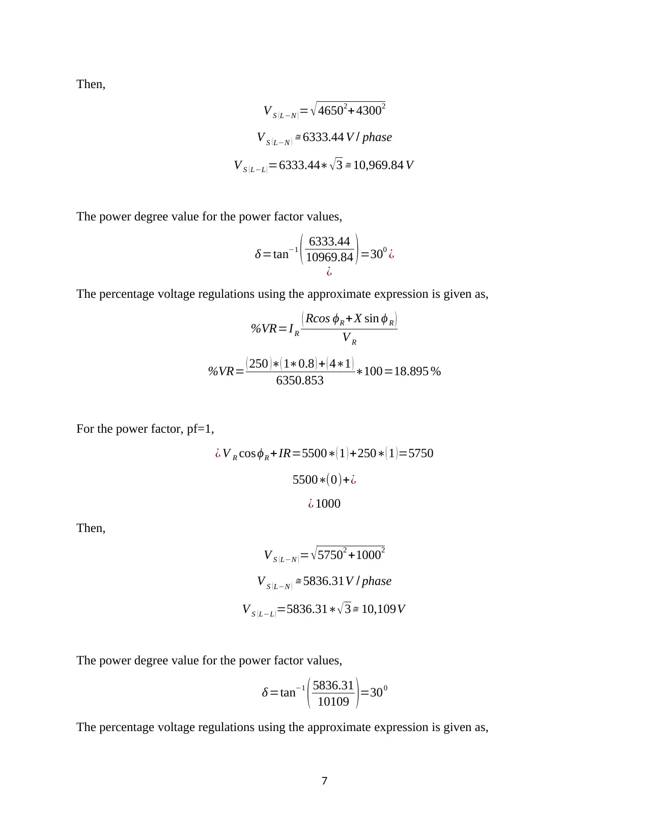
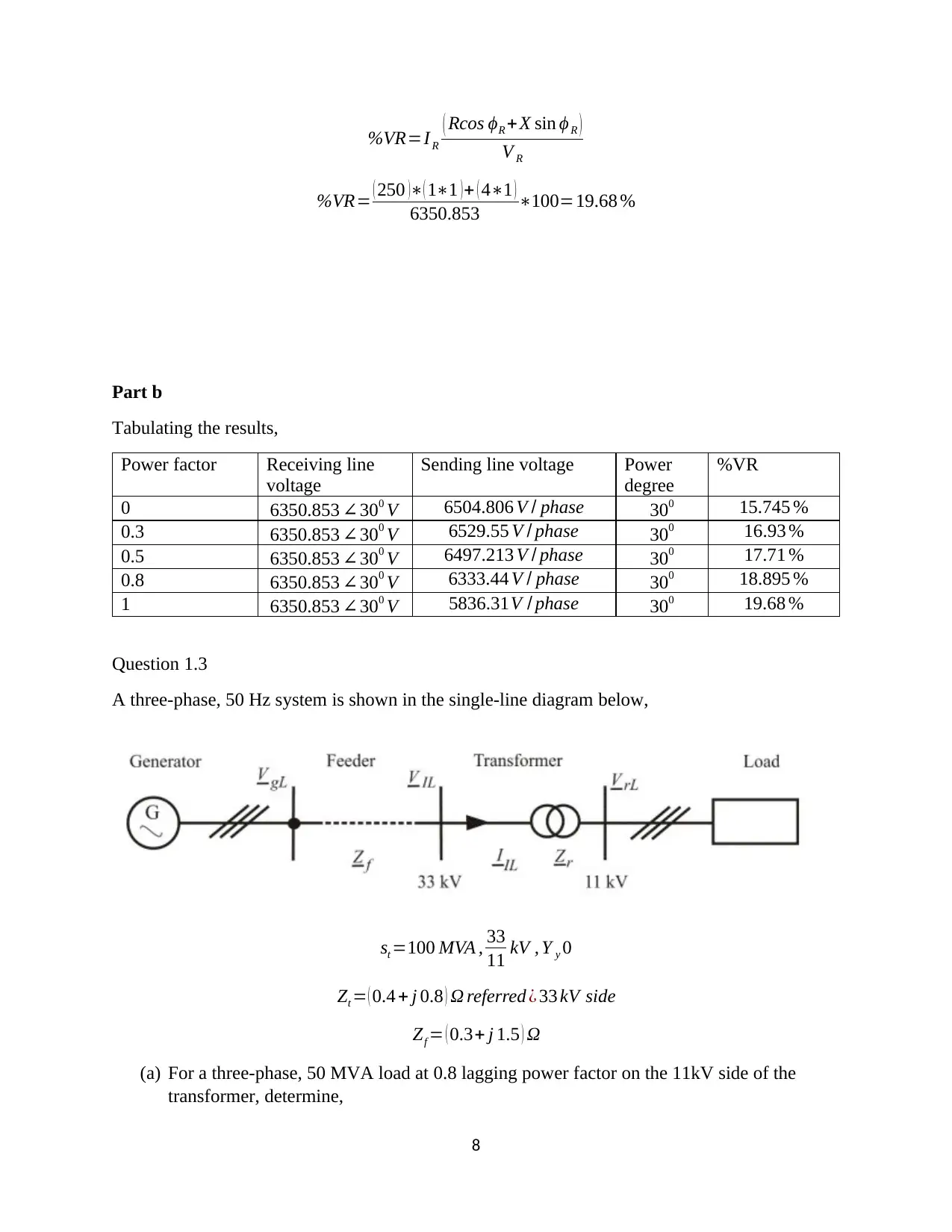
This assignment solution delves into the analysis of short transmission lines, focusing on voltage regulation and power factor. It begins by outlining the equivalent circuit for a short transmission line and then calculates the sending-end voltage, power angle, and voltage regulation for various leading and lagging power factors. The solution further examines the impact of capacitor banks on improving the power factor and analyzes the line currents, generator voltage, complex power output, voltage regulation, and transmission efficiency under different power factor conditions. The document also addresses voltage drop calculations in a distribution network, considering scenarios with and without interconnectors, and evaluates the need for such interconnectors based on allowable voltage drop limits. Desklib offers a wide range of similar solved assignments and past papers to aid students in their studies.

Electrical Power
Student Name
Student ID Number
Institutional Affiliation
Date of submission
1

Question 1.2
Three-phase short transmission line has impedance,
Z= ( R+ jX ) = ( 1+ j 4 ) Ω
phase
(i) Sketch the short-line equivalent circuit per phase and annotate it with the given data
(ii) For a constant receiving-end line voltage, V 2 L=11 kV ∠ 300and line current I =250 A
into a star connected load:
(a) Determine and tabulate for five leading and lagging power factor λ=0,0.8,1:
(i) The sending-end input line voltage (complex/rectangular format)
(ii) The power angle in degrees
(iii) Voltage regulation (%)
(b) Calculate:
(iv) The 5 approximate voltage regulations and tabulate the values using the
approximation
ε va ≈ RIcos ϕ−XI sin ϕ
V 2
SOLUTION
Part i
Transmission lines with a length less than 50 km are the short-line transmission lines.
The capacitance and leakage resistance are negligible in these transmission lines. The two-port
network analogy is implemented. The equivalent short transmission circuit is implemented as,
Z= ( 1+ j 4 ) Ω
phase
2

The phasor diagram of the short transmission line can be referenced to an inductive load or a
capacitive load such that,
Figure 1 Phasor diagram with reference to an inductive load
Figure 2 phasor diagram with reference to a capacitive load
Part ii
Using the V R as the reference, the equation can be written as,
V S =V R + ( IR cos ϕR ± j I R sin ϕ R ) ( R+ j X L )
±−used for lagging∧leading power factor
V S = √ ( V R + IR cos ϕ R + IX sin ϕR ) 2+ ( IX cos ϕR ± IR sin ϕ R )
2
The load angle is given as,
δ =ϕs−ϕ R
Alternatively,
δ=tan−1
( IX cos ϕR ± IR sin ϕR
V R + IR cos ϕR + IX sin ϕR )
3

[V S
I S ]=[ A B
C D ] [V R
IR ]
[ V S
I S ] =[ 1 Z
0 1 ] [ V R
I R ]
[ V R
IR ] = [ 1 −Z
0 1 ] [ V S
I S ]
Voltage regulation
%VR=
|V S|−|V R |
|V R| x 100
It is approximated as,
%VR= R cos ϕR ± X sin ϕR
V R
x 100
Using actual values,
The line current is given as,
I =250 A , Z= (1+ j 4 )
IZ=250∗( 1+ j4 )=250+ j 1000V
The sending-end input line voltage,
V R ( L− N )=V R ( L− L )
√3 = 11∗103 ∠ 300
√3 =6350.853 ∠300 V
V S ( L−N ) =V R ( L−N ) + IZ
¿ 6350.853 ∠300 +250+ j1000 V
V S ( L−N ) =5500+ j3175.43+ 250+ j 1000
V S ( L−N ) =5750+ j 4175.43
In phasor notation,
V S ( L−N ) =7.106 kV ∠35.9850
The power degree is given as
δ=35.9850
Using the alternative method with line current and line voltage as the reference,
4

For the power factor, pf=0,
¿ V R cos ϕR +IR=5500∗( 0 ) +250∗( 1 )=250
5500∗(1)+¿
¿ 6500
Then,
V S (L−N )= √2502 +65002
V S ( L−N ) ≅ 6504.806 V / phase
V S (L−L )=6504.806∗√3 ≅ 11,267 V
The power degree value for the power factor values,
δ=tan−1 ( 6504.806
11267 )
¿
=300 ¿
The percentage voltage regulations using the approximate expression is given as,
%VR=I R
( Rcos ϕR +X sin ϕ R )
V R
%VR= ( 250 )∗( 1∗0 ) + ( 4∗1 )
6350.853 ∗100=15.745 %
For the power factor, pf=0.3,
¿ V R cos ϕR +IR=5500∗( 0.3 ) +250∗( 1 )=1900
5500∗(0.954)+(250∗4)
¿ 6247
Then,
V S ( L−N ) = √ 19002 +62472
V S ( L−N ) ≅ 6529.55 V / phase
V S (L−L )=6529.55∗√3 ≅ 11,310 V
The power degree value for the power factor values,
5

δ=tan−1 ( 6529.55
11310 )
¿
=300 ¿
The percentage voltage regulations using the approximate expression is given as,
%VR=I R
( Rcos ϕR +X sin ϕ R )
V R
%VR= ( 250 )∗( 1∗0.3 ) + ( 4∗1 )
6350.853 ∗100=16.93 %
For the power factor, pf=0.5,
¿ V R cos ϕR + IR=5500∗( 0.5 ) +250∗( 1 ) =3000
5500∗(0.866)+¿
¿ 5763.14
Then,
V S (L−N )= √30002 +5763.142
V S ( L−N ) ≅ 6497.213 V / phase
V S (L−L )=6497.213∗√3 ≅ 11,254 V
The power degree value for the power factor values,
δ =tan−1 ( 6497.123
11254 )
¿
=300 ¿
The percentage voltage regulations using the approximate expression is given as,
%VR=I R
( Rcos ϕR +X sin ϕ R )
V R
%VR= ( 250 )∗( 1∗0.5 ) + ( 4∗1 )
6350.853 ∗100=17.71 %
For the power factor, pf=0.8,
¿ V R cos ϕR +IR=5500∗( 0.8 ) +250∗( 1 )=4650
5500∗(0.6)+¿
¿ 4300
6

Then,
V S (L−N )= √46502+43002
V S (L−N ) ≅ 6333.44 V / phase
V S ( L−L ) =6333.44∗ √ 3 ≅ 10,969.84 V
The power degree value for the power factor values,
δ=tan−1 ( 6333.44
10969.84 )
¿
=300 ¿
The percentage voltage regulations using the approximate expression is given as,
%VR=I R
( Rcos ϕR +X sin ϕ R )
V R
%VR= ( 250 )∗( 1∗0.8 ) + ( 4∗1 )
6350.853 ∗100=18.895 %
For the power factor, pf=1,
¿ V R cos ϕR + IR=5500∗( 1 ) +250∗( 1 ) =5750
5500∗(0)+¿
¿ 1000
Then,
V S ( L−N ) = √ 57502 +10002
V S ( L−N ) ≅ 5836.31V / phase
V S ( L−L ) =5836.31∗√ 3≅ 10,109V
The power degree value for the power factor values,
δ =tan−1
( 5836.31
10109 )=300
The percentage voltage regulations using the approximate expression is given as,
7

%VR=I R
( Rcos ϕR +X sin ϕ R )
V R
%VR= ( 250 )∗( 1∗1 )+ ( 4∗1 )
6350.853 ∗100=19.68 %
Part b
Tabulating the results,
Power factor Receiving line
voltage
Sending line voltage Power
degree
%VR
0 6350.853 ∠300 V 6504.806 V / phase 300 15.745 %
0.3 6350.853 ∠300 V 6529.55 V / phase 300 16.93 %
0.5 6350.853 ∠300 V 6497.213 V / phase 300 17.71 %
0.8 6350.853 ∠300 V 6333.44 V / phase 300 18.895 %
1 6350.853 ∠300 V 5836.31V / phase 300 19.68 %
Question 1.3
A three-phase, 50 Hz system is shown in the single-line diagram below,
st =100 MVA , 33
11 kV , Y y 0
Zt = ( 0.4 + j 0.8 ) Ω referred ¿ 33 kV side
Zf = ( 0.3+ j 1.5 ) Ω
(a) For a three-phase, 50 MVA load at 0.8 lagging power factor on the 11kV side of the
transformer, determine,
8

(i) The kVA rating of the 11-kV delta connected capacitor bank required at the load
to improve the load power factor to unity
(ii) The capacitance per phase.
(b) For the case of 0.8 lagging and unity power factor (capacitors in service) determine and
compare the following quantities
(i) Line currents on the 33kV side
(ii) Line voltage of the generator
(iii) The generator output complex power
(iv) The voltage regulation of the system
(v) The transmission efficiency of the system
SOLUTION
Part a
Kva rating required to maintain the power factor to unity.
( kVA )2= ( kW )2+ ( kVAR )2
The power factor is given as,
cos ϕ= kW
kVA
At the 11-kV delta connected capacitor bank the load value to improve power factor is given as,
1= kW
100 mVA
For a linear connection, the total impedance is given as,
Ztotal =Zf +Zt
Ztotal = ( 0.4+ j 0.8 ) + ( 0.3+ j 1.5 )
Ztotal =0.7+ j2.3 Ω
kVAR=kW ∗tan ϕ
→ ( 11 k ) 2
0.7 =172.857 mVA rating
The capacitor values per phase,
9

Part b
The line current is given as,
I = W
√ 3 Ecos ϕ
A= l
σ =length of the line conductor
current density = W
√3 . E . σ . cos ϕ
R= ρl
A = √ 3 . E . ρι . cos ϕ
W
V lg=33 kV (33 kV
11 kV )=33 kV
V ¿=11 kv ( 11 kV
33 kV )=11 kV
10

Question 1.4
Distribution network voltage drop
(a) Calculate the voltage drop from A to C and the voltages with respect to earth at B, C, D,
and E, when the single-phase distribution network shown below is fed at node A at
V a =240V ∠ 00
(i) With no interconnector between A and C
(ii) With an interconnector of impedance Zac ( ii ) =0.2+ j0.05 Ωbetween A and C
(iii) With an interconnector of impedance Zac ( iii ) =0.1+ j 0.025 Ωbetween A and C
11
I base=100×106
√ 3(230×103 )=251 ⇒ I t=1 . 2475(251)=313 . 1 amperes
It , pu = 1. 0
X x 1 +Zt + X x 2 + RL
= 1 . 0
j 0 . 0191+0 .0004 + j 0 . 005+ j 0 .02+ 0. 8 = 1 .0
0 . 8004+ j0 . 0441 =1. 2456 - j0 . 0686
X pu 2=X pu1⋅
[ V base 1
V base 2 ]
2
⋅
[ Sbase 2
Sbase 1 ]=0. 08⋅[ 19 kV
22 kV ]
2
⋅[ 100 MVA
50 MVA ]=0 . 11934

The distributor section impedances are:
The loads are: 30 A at unity pf at A: 40 A at 0.9 pf lagging at B; 110 A at 0.8 p.f. lagging
at C; 80 A at 0.8 pf lagging at D; and 50 A at unity p.f. at E. all of the loads, and the
current source feeding node A, have a common earth node F.
(b) Between the supply voltage at A and any load point the allowable voltage drop is 4% or
less. Summarize, in matrix format, your load voltage results and briefly comment on
them with respect to the need or otherwise to install an interconnector AC as described
above.
SOLUTION
Part a
Voltage drop per line is given as,
12