ENEL890AO: Regression Experiments for Electrical Engineering Course

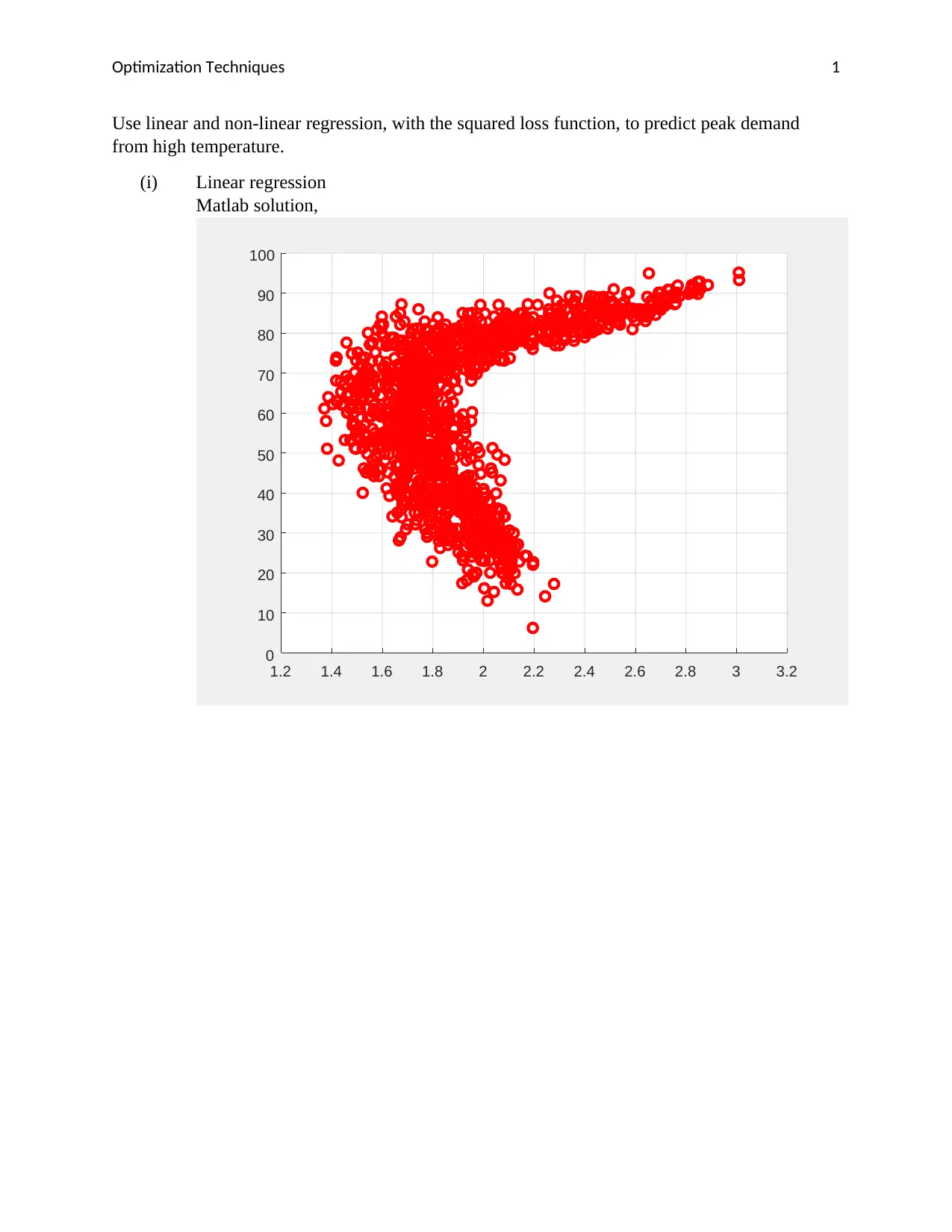
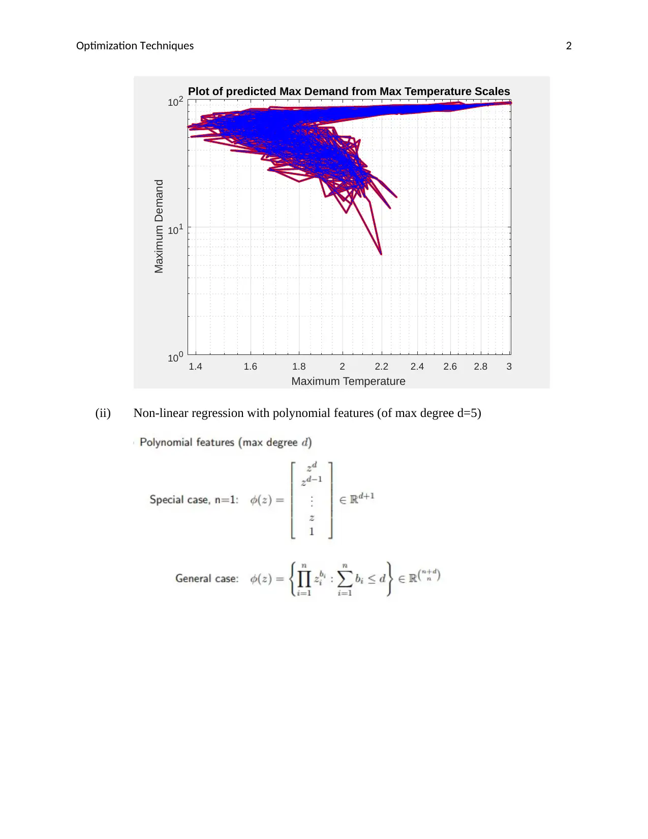
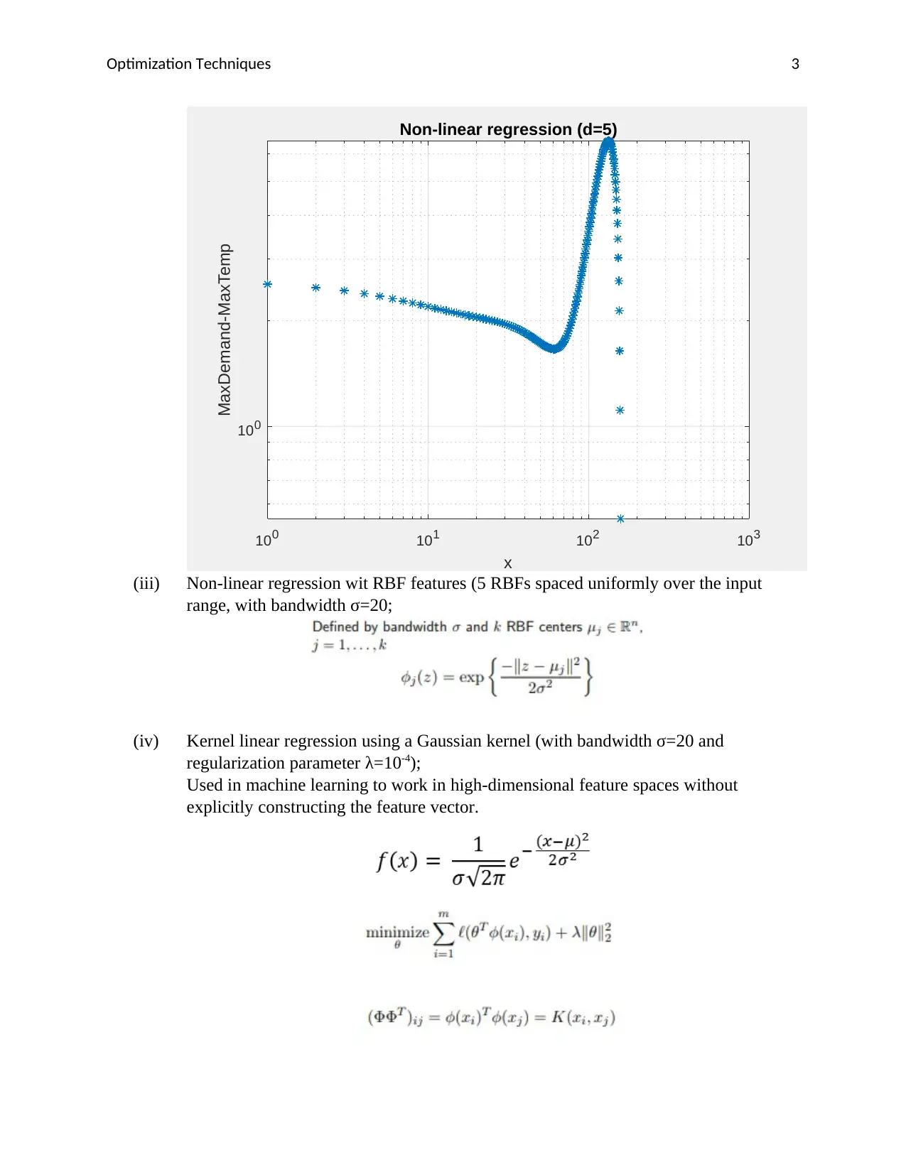
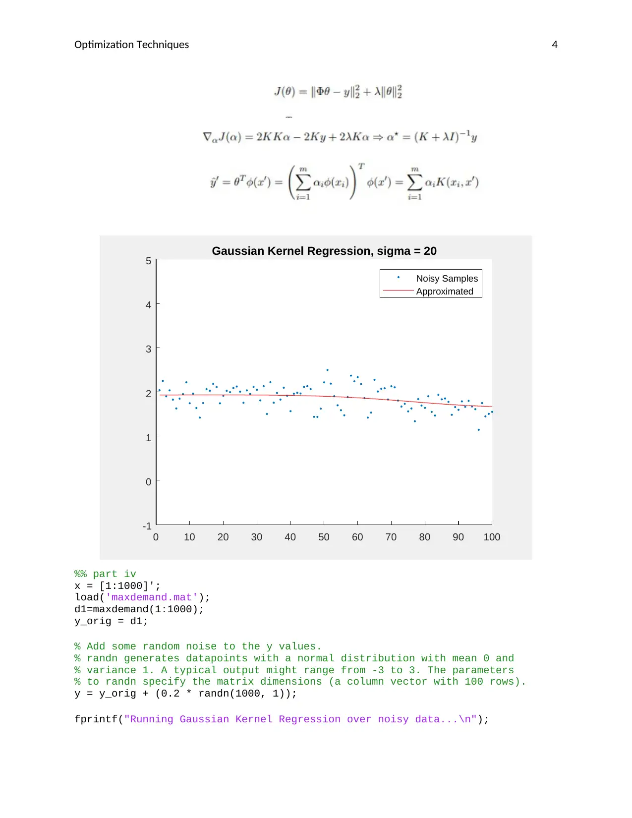
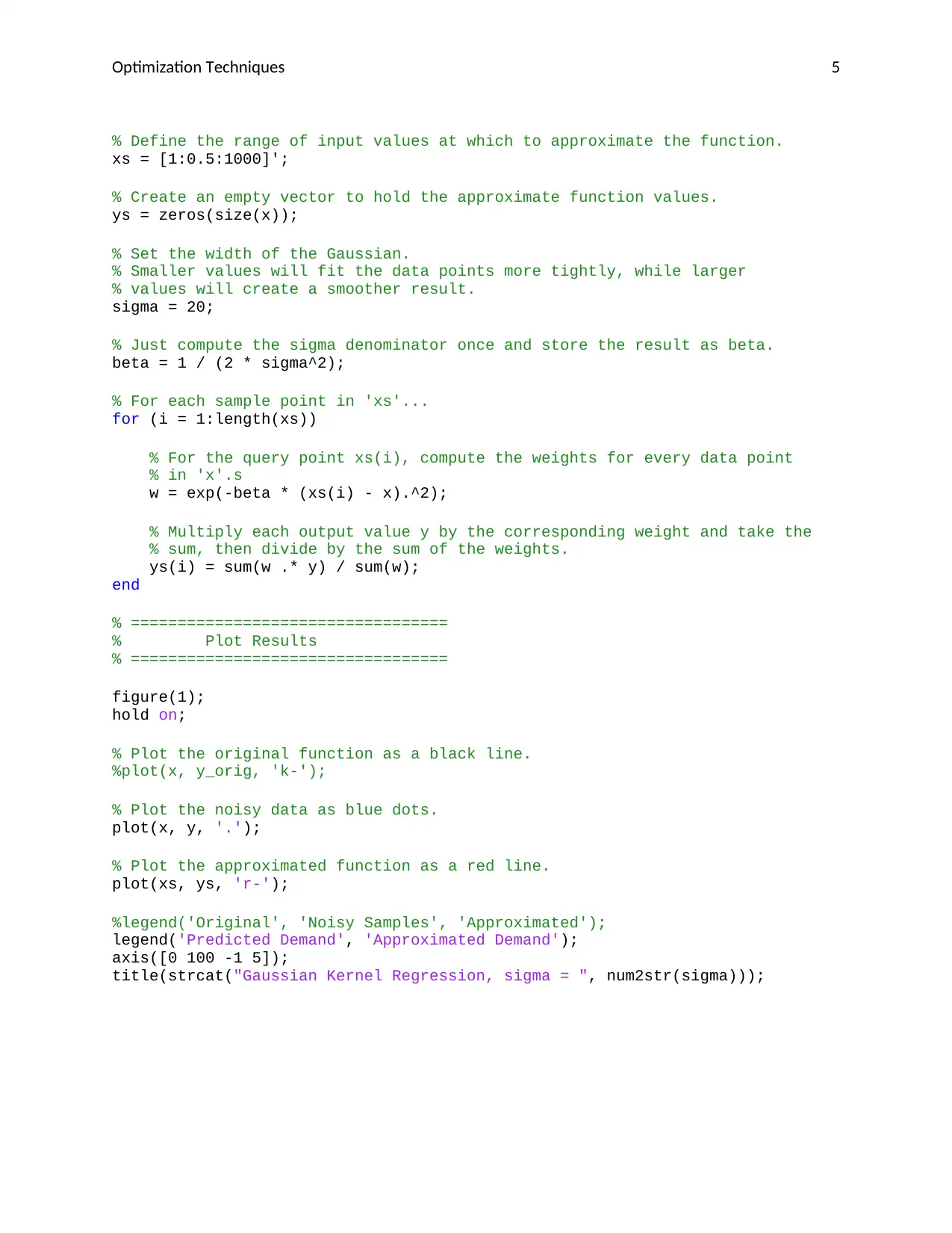
This assignment solution for ENEL890AO Computational Methods in Electrical Engineering focuses on using linear and non-linear regression techniques to predict peak demand from high temperature. The solution implements linear regression, non-linear regression with polynomial features (degree 5), non-linear regression with RBF features, and kernel linear regression using a Gaussian kernel. The code and resulting figures are included, demonstrating the application of these methods and the resulting fits over the input data. The assignment uses the squared loss function for optimization and provides a detailed implementation of Gaussian Kernel Regression over noisy data, including the generation of noisy data points and the approximation of the function with a Gaussian kernel. The results are plotted to visualize the predicted demand and the approximated demand.

2018
INSTITUTIONAL AFFILIATION
FACULTY OR DEPARTMENT
ENEL890AO
COMPUTATIONAL METHODS IN ELECTRICAL
ENGINEERING
TITLE:
ASSIGNMENT 5
EXPERIMENTS WITH LINEAR AND NON-LINEAR
REGRESSION
STUDENT NAME
STUDENT ID NUMBER
DATE OF SUBMISSION

Optimization Techniques 1
Use linear and non-linear regression, with the squared loss function, to predict peak demand
from high temperature.
(i) Linear regression
Matlab solution,
1.2 1.4 1.6 1.8 2 2.2 2.4 2.6 2.8 3 3.2
0
10
20
30
40
50
60
70
80
90
100

Optimization Techniques 2
1.4 1.6 1.8 2 2.2 2.4 2.6 2.8 3
Maximum Temperature
100
101
102
Maximum Demand
Plot of predicted Max Demand from Max Temperature Scales
(ii) Non-linear regression with polynomial features (of max degree d=5)

Optimization Techniques 3
100 101 102 103
x
100
MaxDemand-MaxTemp
Non-linear regression (d=5)
(iii) Non-linear regression wit RBF features (5 RBFs spaced uniformly over the input
range, with bandwidth σ=20;
(iv) Kernel linear regression using a Gaussian kernel (with bandwidth σ=20 and
regularization parameter λ=10-4);
Used in machine learning to work in high-dimensional feature spaces without
explicitly constructing the feature vector.

Optimization Techniques 4
0 10 20 30 40 50 60 70 80 90 100
-1
0
1
2
3
4
5 Gaussian Kernel Regression, sigma = 20
Noisy Samples
Approximated
%% part iv
x = [1:1000]';
load('maxdemand.mat');
d1=maxdemand(1:1000);
y_orig = d1;
% Add some random noise to the y values.
% randn generates datapoints with a normal distribution with mean 0 and
% variance 1. A typical output might range from -3 to 3. The parameters
% to randn specify the matrix dimensions (a column vector with 100 rows).
y = y_orig + (0.2 * randn(1000, 1));
fprintf("Running Gaussian Kernel Regression over noisy data...\n");

Optimization Techniques 5
% Define the range of input values at which to approximate the function.
xs = [1:0.5:1000]';
% Create an empty vector to hold the approximate function values.
ys = zeros(size(x));
% Set the width of the Gaussian.
% Smaller values will fit the data points more tightly, while larger
% values will create a smoother result.
sigma = 20;
% Just compute the sigma denominator once and store the result as beta.
beta = 1 / (2 * sigma^2);
% For each sample point in 'xs'...
for (i = 1:length(xs))
% For the query point xs(i), compute the weights for every data point
% in 'x'.s
w = exp(-beta * (xs(i) - x).^2);
% Multiply each output value y by the corresponding weight and take the
% sum, then divide by the sum of the weights.
ys(i) = sum(w .* y) / sum(w);
end
% ==================================
% Plot Results
% ==================================
figure(1);
hold on;
% Plot the original function as a black line.
%plot(x, y_orig, 'k-');
% Plot the noisy data as blue dots.
plot(x, y, '.');
% Plot the approximated function as a red line.
plot(xs, ys, 'r-');
%legend('Original', 'Noisy Samples', 'Approximated');
legend('Predicted Demand', 'Approximated Demand');
axis([0 100 -1 5]);
title(strcat("Gaussian Kernel Regression, sigma = ", num2str(sigma)));