Electrical Engineering Assignment: Unit 6 Tasks Analysis

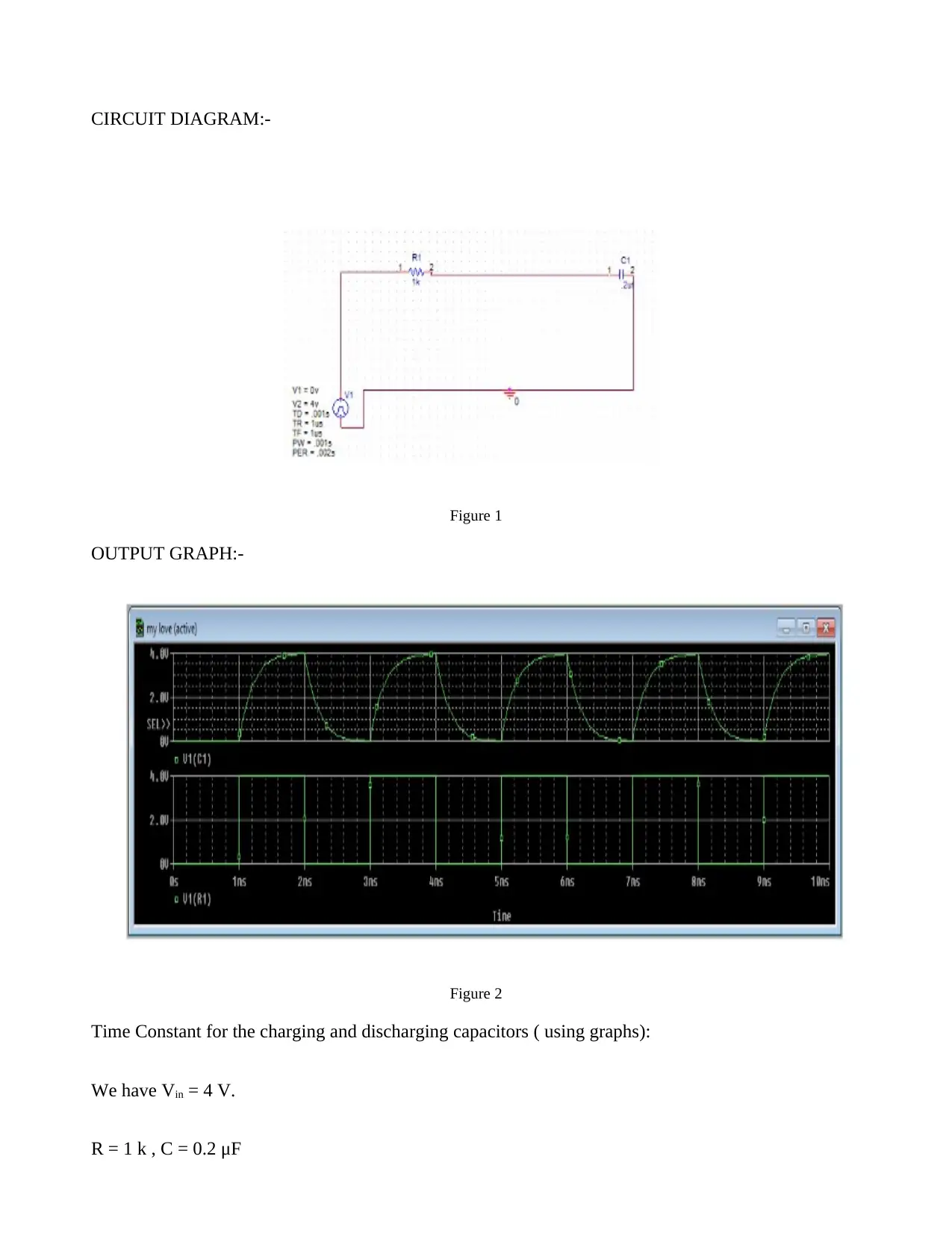
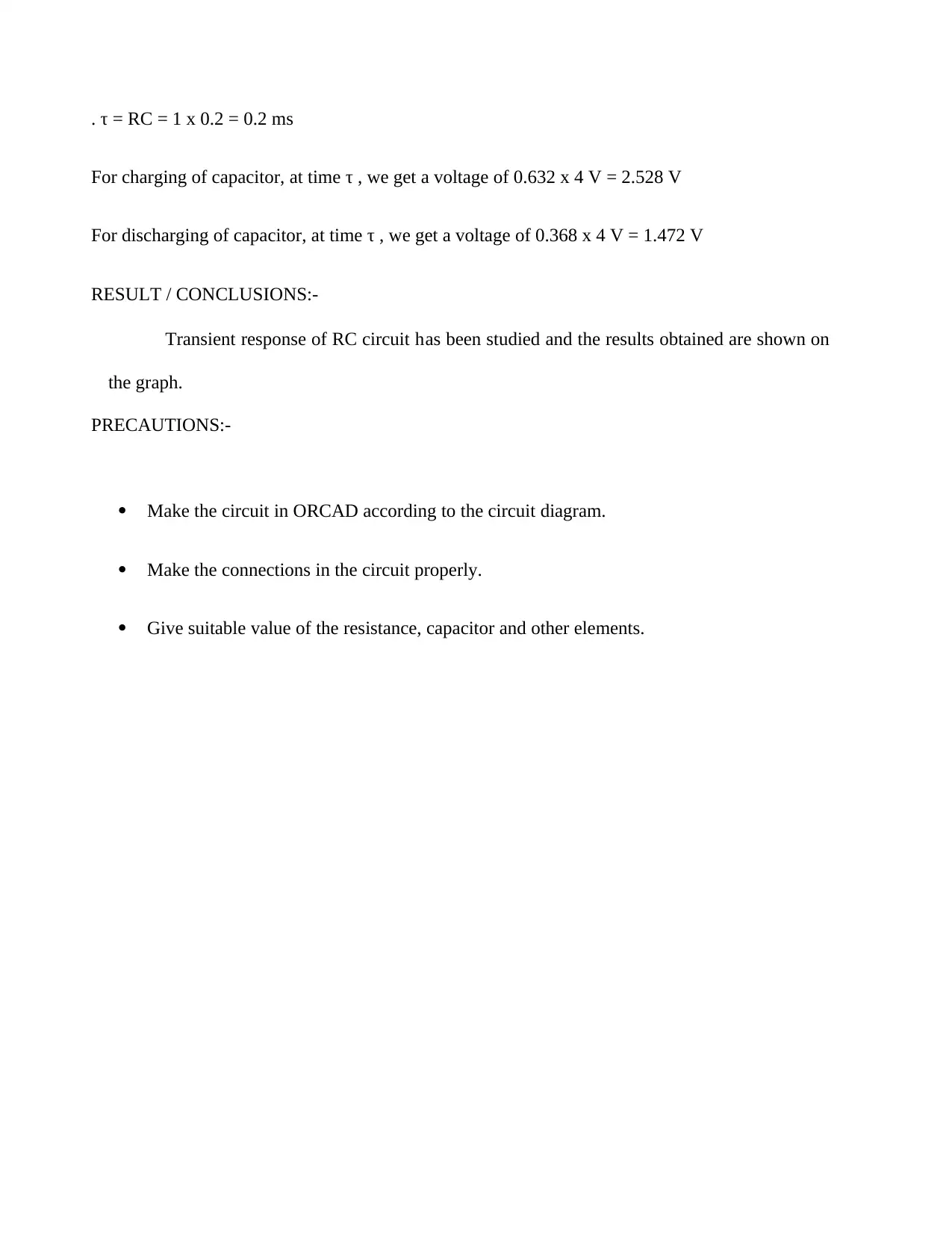
This electrical engineering assignment presents a comprehensive analysis of various electrical concepts and principles. The assignment begins with an experiment using P-Spice software to study the transient response of an RC circuit, including circuit creation, simulation setup, and result analysis. It then delves into capacitor analysis, solving problems involving series and parallel capacitor configurations, calculating equivalent capacitance, charge, voltage, and energy stored. The assignment also explores magnetism, discussing BH curves for iron and steel, their relationship, and the application of silicon steel in transformer cores. Furthermore, the assignment examines the impact of legislation on engineering companies, discussing its effects on operations, employee-employer relationships, and the creation of safe working environments. The assignment also covers sinusoidal AC signals, oscilloscope signals, and the operation and effects of varying component parameters in a power supply circuit. The assignment is well-structured, providing detailed solutions, calculations, and explanations for each task.

Electrical Assignment
Student Name –
Student ID -

Contents
TASK 2:..................................................................................................................................................................3
EXPERIMENT.....................................................................................................................................................3
TASK 3:..................................................................................................................................................................8
TASK 4:................................................................................................................................................................11
Unit 6 Task 2........................................................................................................................................................12
Task: Legislation..................................................................................................................................................13
Task 1..................................................................................................................................................................14
References..........................................................................................................................................................20

TASK 2:
We have to carry out an experiment to determine the relationship between the voltage and current for
charging and discharging capacitor.
EXPERIMENT
OBJECTIVE:-
To study and plot the transient response of RC circuit using P-Spice software.
APPARATUS REQUIRED:-
Computer system and P-Spice software
BRIEF THEORY:-
Applying Kirchhoff’s voltage low to the circuit shown in figure,
1 / C ∫ i dt + R . i = V
Differentiating w.r.t ‘t’
1 / C i + R di / dt = 0
R di / dt = -1 / C . i
.di / i = 1 / RC dt
Integrating w.r.t to’i’ on L.H.S. and w.r.t. ‘t’ on R.H.S. and then taking log on both sides
Log i = -1/RC t + log c
or i=c e-t/RC

On putting I = V/R in above equation, we get
V/R=c e-t/RC At t = 0 , c = V/R
Thus i=V/R e-t/RC
PROCEDURE:-
STEP1-CIRCUIT CREATION WITH CAPTURE
 Open the PSpice software and create a new analog , mixed AD project.
 Select the circuit parts from the respective libraries and place them in the circuit.
 Connect the parts using wire.
 Specify the values and names of the circuit elements ( R = 1 k, C = 0.2 μF ).
STEP2:-SPECIFY TYPE OF SIMULATION
 Create a simulation profile.
 Select the time domain analysis.
 Now run PSpice.
STEP3:-VIEW THE RESULT
 Now select the Traces menu to add traces to the probe window.
 Select V (R1) and V (C1) for the output responses of the resistor and the capacitor.

CIRCUIT DIAGRAM:-
Figure 1
OUTPUT GRAPH:-
Figure 2
Time Constant for the charging and discharging capacitors ( using graphs):
We have Vin = 4 V.
R = 1 k , C = 0.2 μF

. τ = RC = 1 x 0.2 = 0.2 ms
For charging of capacitor, at time τ , we get a voltage of 0.632 x 4 V = 2.528 V
For discharging of capacitor, at time τ , we get a voltage of 0.368 x 4 V = 1.472 V
RESULT / CONCLUSIONS:-
Transient response of RC circuit has been studied and the results obtained are shown on
the graph.
PRECAUTIONS:-
 Make the circuit in ORCAD according to the circuit diagram.
 Make the connections in the circuit properly.
 Give suitable value of the resistance, capacitor and other elements.

Charging:
Let us consider a series RC circuit which is connected to a voltage V.
The KVL equation gives:
V – Q / C – R dQ / dt = 0
Q = Qf ( 1 – e –t / RC )
Qf = Final charge on capacitor at infinite time.
Time Constant = τ = Time at which the charge becomes 0.632 Qf
. τ = RC
Time constant is the time required for charge on the charging capacitor to rise to 63
% of its final value.
Q = Qf ( 1 – e – RC / RC ) = Qf ( 1 – e -1 ) = 0.632 Qf
Discharging:
Let us consider a capacitor charged to a value of Qo connected to a resistance R in
series. This capacitor will slowly discharge.
The KVL equation gives :
Q / C – R dQ / dt = 0
Q = Qo e – t / RC
Time Constant = τ = Time at which the charge remains 0.368 Qo
Time constant is the time required for charge on the discharging capacitor to fall to
36.8 % of its initial value.
Q = Qo e - t / RC = Qo e -1 = 0.368 Qo
We find that the results obtained theretically by calculation and the results obtained by
experiment are the same .

TASK 3:
Solution:
In this case, the capacitors are connected in series.
Let the equivalent capacitance be Ceq
1 / Ceq = 1 / C1 + 1 / C2 + 1 / C3
= 1/12 + 1/3 + 1/6 = 7/12
Ceq = 12/7 μ F
V = 350 V
Total Charge = Q = Ceq . V = 12/7 x 350 = 600 μC
Charge is same for all the 3 capacitors as they are connected in series.
V1 = Q / C1 = 600 / 12 = 50 V
V2 = Q / C2 = 600 / 3 = 200 V
V3 = Q / C3 = 600 / 6 = 100 V

Energy = E = ½ CV2 = ½ QV
E1 = ½ QV1 = ½ x 600 x 50 = 15 mJ
E2 = ½ QV2 = ½ x 600 x 200 = 60 mJ
E3 = ½ QV3 = ½ x 600 x 100 = 30 mJ
Solution:
In this case, the capacitors are connected in parallel.
Let the equivalent capacitance be Ceq
Ceq = C1 + C2 + C3
= 0.1 + 0.2 + 0.3
Ceq = 0.6 μ F
V = 12 V

Voltage is same for all the 3 capacitors as they are connected in parallel.
Q1 = C1 . V = 0.1 x 12 = 1.2 μC
Q2 = C2 . V = 0.2 x 12 = 2.4 μC
Q3 = C3 . V = 0.3 x 12 = 3.6 μC
Energy = E = ½ CV2 = ½ QV
E1 = ½ Q1V = ½ x 1.2 x 12 = 7.2 μJ
E2 = ½ Q2V = ½ x 2.4 x 12 = 14.4 μJ
E3 = ½ Q3V = ½ x 3.6 x 12 = 21.6 μJ

TASK 4:
Total Capacitance = Ceq
C4 = C1 + C2 = 3 + 2 = 5 μF
1 / Ceq = 1 / C4 + 1 / C3 = 1 / 5 + 1 / 15
Ceq = 15 / 4 μF
Total Voltage ,V = 240 V
Total Charge, Q = Ceq . V = 15 / 4 x 240 = 900 μC = Q3 ( Since charge is same in series)
Energy, E3 = ½ Q32/C3 = ½ x 9002 / 15 = 27 mJ
V3 = Q3 / C3 = 900 / 15 = 60 V
V1 = V2 = V – V3 = 240 – 60 = 180 V ( Voltage is same for parallel components )
Q1 = C1 . V1= 3 x 180 = 540 μC
Q2 = C2 . V2 = 2x 180 = 360 μC

E1 = ½ C1V12 = ½ x 3 x 180 x 180 = 0.0486 J
E2 = ½ C2V22 = ½ x 2 x 180 x 180 = 0.0324 J
Unit 6 Task 2
Magnetism Assignment
We are given the graphs of magnetic field strength ( H ) and flux density ( B ) for iron and
steels. These are called the BH curves and they demonstrate the magnetic properties of a
material.
Relationship between flux density ( B ) and field strength ( H ) in BH curves
The graph shows that as the magnetic field strength ( H ) increases the magnetic flux density
( B ) also increases in the material. But a point comes when a further increase in H brings