Principles, Laws, and Applications of Electromagnetic Devices
VerifiedAdded on 2023/02/01
|17
|4429
|45
Report
AI Summary
This report provides a comprehensive overview of electromagnetic devices, beginning with an introduction to scalar and vector fields, fundamental concepts essential for understanding electromagnetic phenomena. It then delves into Coulomb's law, explaining electrostatic forces between charged particles, and Gauss's law, which relates electric charge distribution to the resulting electric field. The report differentiates between permanent and electromagnets, highlighting their characteristics and applications. Furthermore, it discusses the Bio-Savart law, Ampere force law, and the toroidal coil, providing insights into their principles and practical implementations. Numerical examples are included to illustrate the application of these laws and concepts. Overall, the report offers a detailed analysis of the principles and applications of electromagnetic devices, covering essential topics in electrical engineering.
Electromagnetic devices
Paraphrase This Document
Need a fresh take? Get an instant paraphrase of this document with our AI Paraphraser
TABLE OF CONTENTS
INTRODUCTION...........................................................................................................................1
1. Scalar and vector fields ...........................................................................................................1
2. Coulomb's law .........................................................................................................................2
Vector form of coulombs-law......................................................................................................3
3. Gauss law ................................................................................................................................5
4. Permanent and electromagnets ...............................................................................................8
5. Bio- Savart law .......................................................................................................................9
6. Ampere force law ..................................................................................................................10
7. Toroisal coil ..........................................................................................................................11
CONCLUSION .............................................................................................................................13
REFERENCES .............................................................................................................................14
INTRODUCTION
Electromagnetic devices are based upon the principles of electric and magnetic
interaction as varying electric fields produces magnetic field and vice versa. The report will
discuss the various concepts and laws on which electromagnetic devices work upon.
1. Scalar and vector fields
Scalar quantities are defined as the entities which are characterised by magnitude only
and does not have any specific direction. On the other hand vector quantitate are known to be
entities with both direction and magnitude. For instance quantities like electric charge, distance
and mass are called scalar while velocity, displacement and magnetic fields are vectors (Jiles,
2015). In electromagnetic theory fields are defined as the quantities which are function of
position and may also depends upon time or other customised variables.
On the basis of nature of quantities fields are classified as scalar or vector fields. For
example temperature is scalar quantity and temperature distribution in any rod is scalar field
because at every point in the specified region of rod scalar function has defined value. Similarly,
in velocity filed of moving object at every location value of vector function is defined so that the
entire region is known as vector field.
Use and practical implementation:
Both scalar and vector fields are employed and analysed for variety of applications and
purpose. Vector fields are used in modelling the directional and magnitude aspects of fluids or
the physical quantities such as force or velocity. These fields are also an integral part of integral
and differential calculus (Tran, 2018). For instance this usage of vector field is implemented in
determining work done, interpretation of energy conservation, flow rotation (curl) and changes in
fluid flow volume (divergence). Along with the vectors, scalar fields are also used in quantum
theory and to underpin the applications based upon theory of relativity.
The distribution of scalar quantities such as spin zero, temperature and pressure
distribution within space or different objects be determined only with the application of scalar
and vector operations. The fields such as electric potential or gravitational forces cannot be
described without discussion of implementation of scalar and vector fields. The scalar quantities
are used in meteorology while the vector fields find their application in the electromagnetic
devices (Farrow, 2019).
Numerical example:
1
⊘ This is a preview!⊘
Do you want full access?
Subscribe today to unlock all pages.
Trusted by 1+ million students worldwide
To determine the maximum rate of change in any scalar quantity in a particular direction
gradient of scalar quantity is used. For instance the maximum change in function z= 4x²+ siny
+6z can be calculated by determining its gradient as follows:
Gradient z= z = (∂z/∂x)i + (∂z/∂y)j +(∂z/∂z)k∇
On substituting value of z we get:
z = 8xi +(cosy)j + 6k∇
Similarly, the divergence of any vector quantity can help to find the density variations at any
point. For instance the fluid flow of any liquid represented by vector field equation
u= 4xi + 12y³j +8z²k then its divergence can be calculated by the following formula.
Divergence u= .u = (∂u/∂x)i + (∂u/∂y)j +(∂u/∂z)k∇ (Zohuri, 2019)
.u = 4+ 36y² + 16z∇
This magnitude of this obtained vector provides the maximum change in density.
In this way various operations of scalar and vector quantities helps to determine the rotational
and linear motion properties of physical quantities.
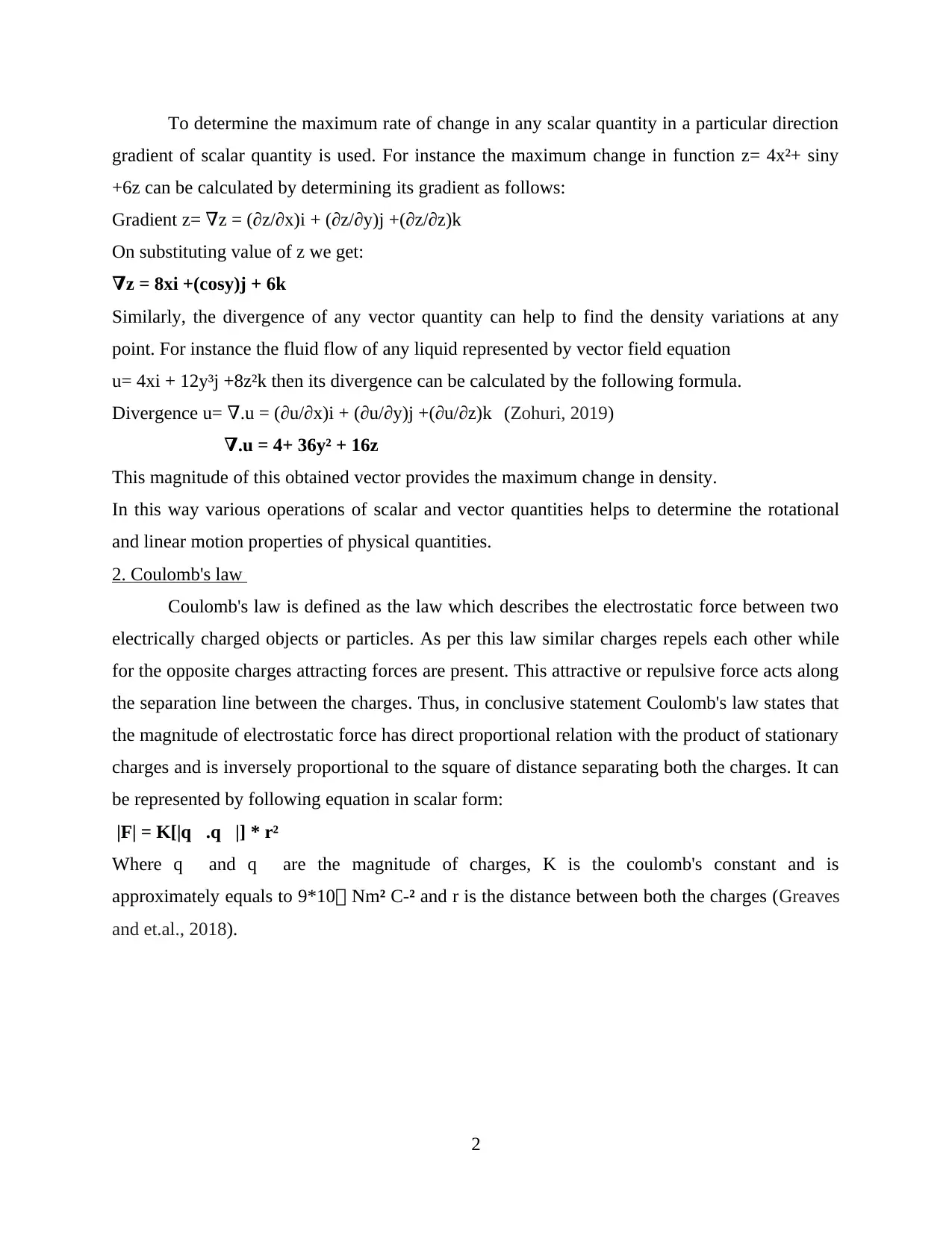
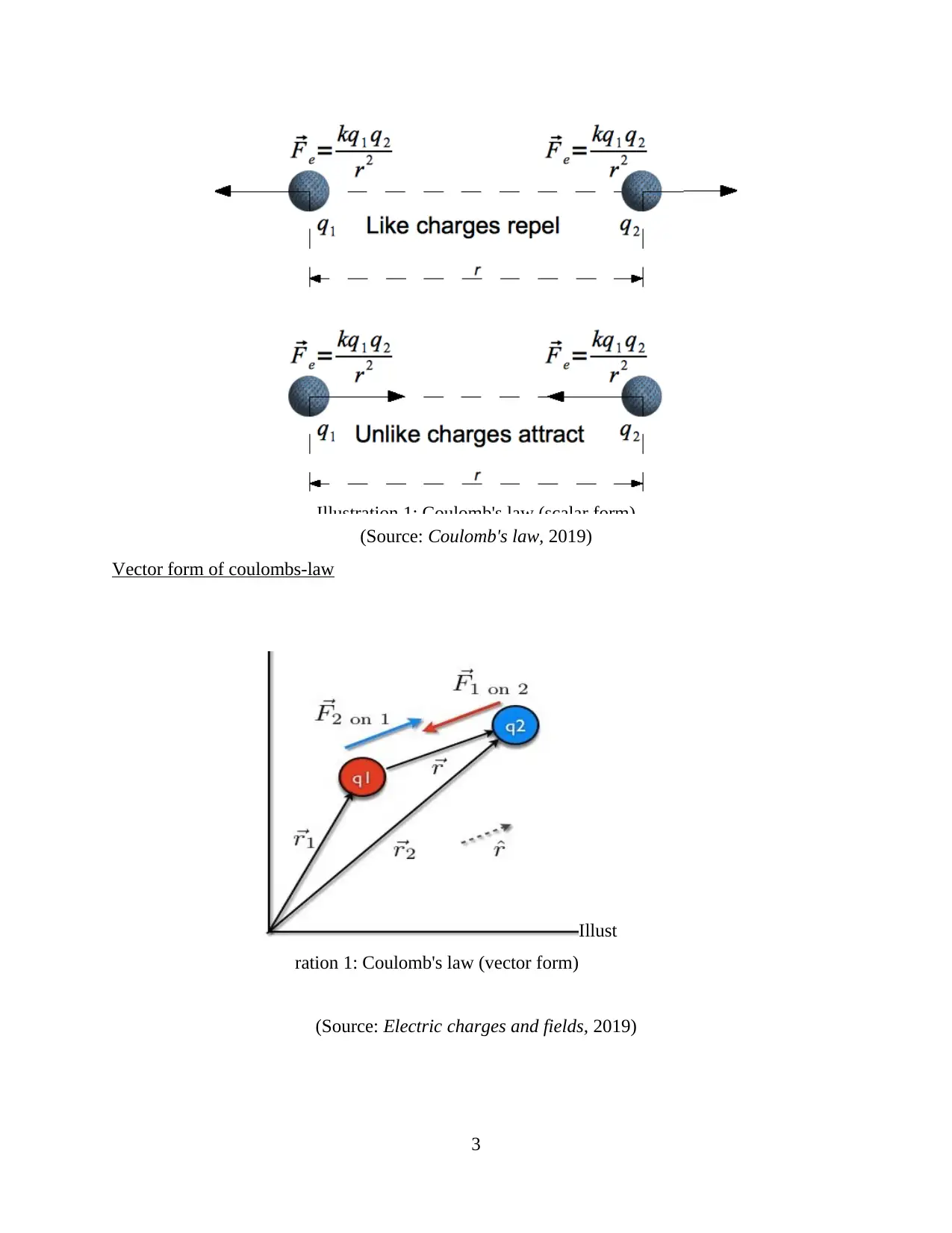
2. Coulomb's law
Coulomb's law is defined as the law which describes the electrostatic force between two
electrically charged objects or particles. As per this law similar charges repels each other while
for the opposite charges attracting forces are present. This attractive or repulsive force acts along
the separation line between the charges. Thus, in conclusive statement Coulomb's law states that
the magnitude of electrostatic force has direct proportional relation with the product of stationary
charges and is inversely proportional to the square of distance separating both the charges. It can
be represented by following equation in scalar form:
|F| = K[|q.q|] * r²
Where q and q are the magnitude of charges, K is the coulomb's constant and is
approximately equals to 9*10 Nm² C-² and r is the distance between both the charges (Greaves
and et.al., 2018).
2
gradient of scalar quantity is used. For instance the maximum change in function z= 4x²+ siny
+6z can be calculated by determining its gradient as follows:
Gradient z= z = (∂z/∂x)i + (∂z/∂y)j +(∂z/∂z)k∇
On substituting value of z we get:
z = 8xi +(cosy)j + 6k∇
Similarly, the divergence of any vector quantity can help to find the density variations at any
point. For instance the fluid flow of any liquid represented by vector field equation
u= 4xi + 12y³j +8z²k then its divergence can be calculated by the following formula.
Divergence u= .u = (∂u/∂x)i + (∂u/∂y)j +(∂u/∂z)k∇ (Zohuri, 2019)
.u = 4+ 36y² + 16z∇
This magnitude of this obtained vector provides the maximum change in density.
In this way various operations of scalar and vector quantities helps to determine the rotational
and linear motion properties of physical quantities.
2. Coulomb's law
Coulomb's law is defined as the law which describes the electrostatic force between two
electrically charged objects or particles. As per this law similar charges repels each other while
for the opposite charges attracting forces are present. This attractive or repulsive force acts along
the separation line between the charges. Thus, in conclusive statement Coulomb's law states that
the magnitude of electrostatic force has direct proportional relation with the product of stationary
charges and is inversely proportional to the square of distance separating both the charges. It can
be represented by following equation in scalar form:
|F| = K[|q.q|] * r²
Where q and q are the magnitude of charges, K is the coulomb's constant and is
approximately equals to 9*10 Nm² C-² and r is the distance between both the charges (Greaves
and et.al., 2018).
2
Paraphrase This Document
Need a fresh take? Get an instant paraphrase of this document with our AI Paraphraser
(Source: Coulomb's law, 2019)
Vector form of coulombs-law
(Source: Electric charges and fields, 2019)
3
Illustration 1: Coulomb's law (scalar form)
Illust
ration 1: Coulomb's law (vector form)
Vector form of coulombs-law
(Source: Electric charges and fields, 2019)
3
Illustration 1: Coulomb's law (scalar form)
Illust
ration 1: Coulomb's law (vector form)
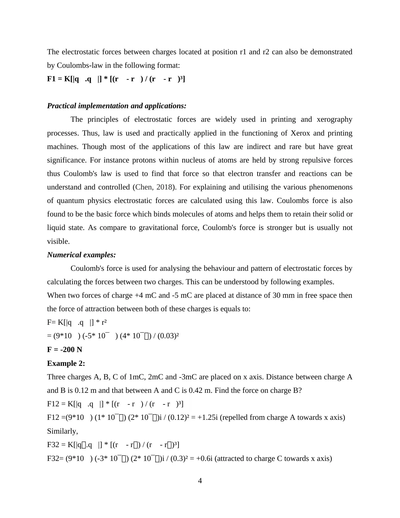
The electrostatic forces between charges located at position r1 and r2 can also be demonstrated
by Coulombs-law in the following format:
F1 = K[|q.q|] * [(r - r) / (r - r)³]
Practical implementation and applications:
The principles of electrostatic forces are widely used in printing and xerography
processes. Thus, law is used and practically applied in the functioning of Xerox and printing
machines. Though most of the applications of this law are indirect and rare but have great
significance. For instance protons within nucleus of atoms are held by strong repulsive forces
thus Coulomb's law is used to find that force so that electron transfer and reactions can be
understand and controlled (Chen, 2018). For explaining and utilising the various phenomenons
of quantum physics electrostatic forces are calculated using this law. Coulombs force is also
found to be the basic force which binds molecules of atoms and helps them to retain their solid or
liquid state. As compare to gravitational force, Coulomb's force is stronger but is usually not
visible.
Numerical examples:
Coulomb's force is used for analysing the behaviour and pattern of electrostatic forces by
calculating the forces between two charges. This can be understood by following examples.
When two forces of charge +4 mC and -5 mC are placed at distance of 30 mm in free space then
the force of attraction between both of these charges is equals to:
F= K[|q.q|] * r²
= (9*10) (-5* 10¯) (4* 10¯) / (0.03)²
F = -200 N
Example 2:
Three charges A, B, C of 1mC, 2mC and -3mC are placed on x axis. Distance between charge A
and B is 0.12 m and that between A and C is 0.42 m. Find the force on charge B?
F12 = K[|q.q|] * [(r - r) / (r - r)³]
F12 =(9*10) (1* 10¯) (2* 10¯)i / (0.12)² = +1.25i (repelled from charge A towards x axis)
Similarly,
F32 = K[|q.q|] * [(r - r) / (r - r)³]
F32= (9*10) (-3* 10¯) (2* 10¯)i / (0.3)² = +0.6i (attracted to charge C towards x axis)
4
⊘ This is a preview!⊘
Do you want full access?
Subscribe today to unlock all pages.
Trusted by 1+ million students worldwide
Thus, resultant force on charge B is = 1.25i +0.6i = 1.85N (In positive x direction)
3. Gauss law
Gauss law is defined as the theorem which gives the relation between electric charge
distribution to resulting electric field within a closed surface such as sphere or cylinder.
According to this law total electric flux within closed surface is equals to the ratio of charge
enclosed by the surface and the permittivity. Electric flux is known as the product of electric
field and surface area which is projected normally to electric field. Gauss law is applicable to
closed surface and allows the evaluation of enclosed charge by the method of electric field
mapping on surface exterior to charge distribution (Nousiainen and Koponen, 2017). Though
Gauss law can be used to find the electric field in variety of symmetical shapes but it cannot be
applied in some specific cases. For instance this law cannot provide the electric field caused by
electric dipoles.
Expression for the Gauss law: ϕ =q/ ϵ₀
Application:
This law is applied and is used to determine the electric fields when the electric charge is
distributed in a continuous pattern within symmetrical objects. Gauss law provides solution for
the complex electrostatic difficulties which can involve planar, spherical or cylindrical
symmetry. The law posses several forms and can be easily converted into differential equations
which makes it solution very easy and simplified. In various practical applications Gauss law
equations are used as solution for the Poission equation and Maxwell's four equations. Gauss law
is also used to find the electric field through various surfaces (Rothwell and Cloud, 2018). The
key applications of this use are as follows:
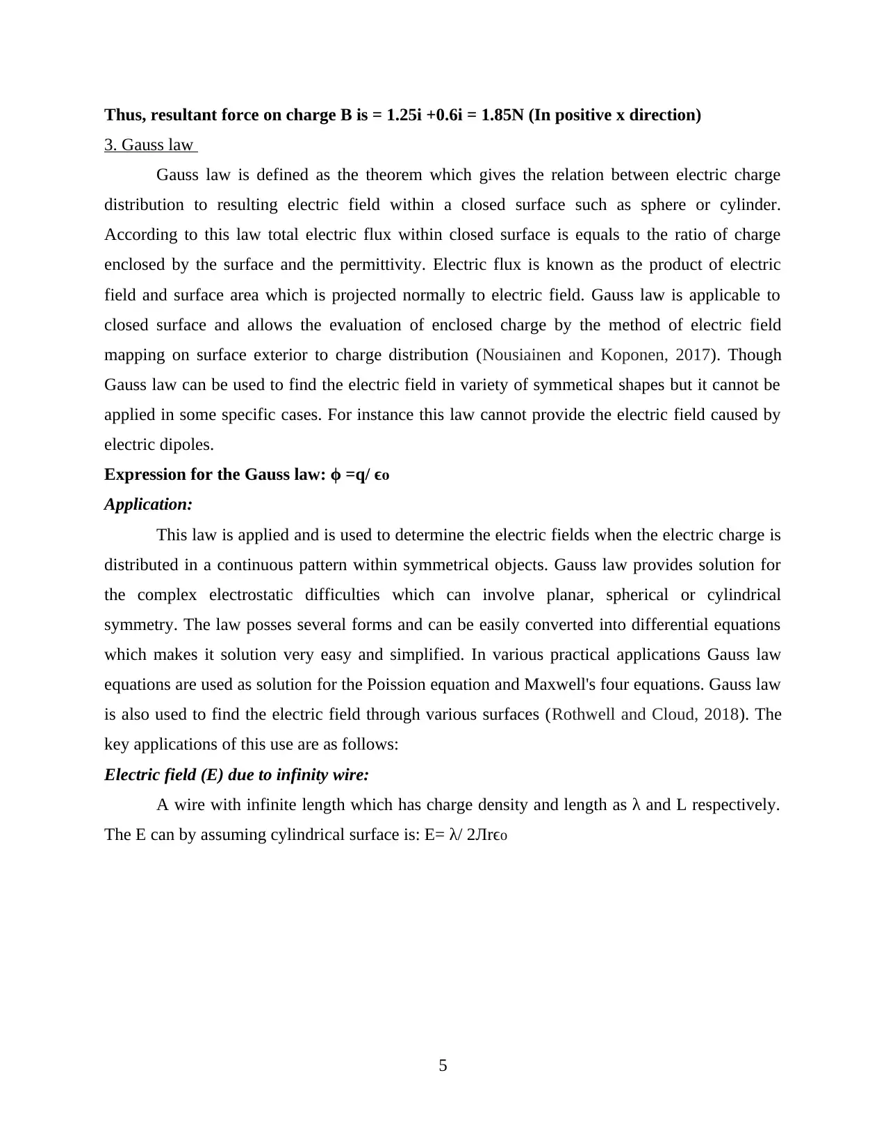
Electric field (E) due to infinity wire:
A wire with infinite length which has charge density and length as λ and L respectively.
The E can by assuming cylindrical surface is: E= λ/ 2Лrϵ₀
5
3. Gauss law
Gauss law is defined as the theorem which gives the relation between electric charge
distribution to resulting electric field within a closed surface such as sphere or cylinder.
According to this law total electric flux within closed surface is equals to the ratio of charge
enclosed by the surface and the permittivity. Electric flux is known as the product of electric
field and surface area which is projected normally to electric field. Gauss law is applicable to
closed surface and allows the evaluation of enclosed charge by the method of electric field
mapping on surface exterior to charge distribution (Nousiainen and Koponen, 2017). Though
Gauss law can be used to find the electric field in variety of symmetical shapes but it cannot be
applied in some specific cases. For instance this law cannot provide the electric field caused by
electric dipoles.
Expression for the Gauss law: ϕ =q/ ϵ₀
Application:
This law is applied and is used to determine the electric fields when the electric charge is
distributed in a continuous pattern within symmetrical objects. Gauss law provides solution for
the complex electrostatic difficulties which can involve planar, spherical or cylindrical
symmetry. The law posses several forms and can be easily converted into differential equations
which makes it solution very easy and simplified. In various practical applications Gauss law
equations are used as solution for the Poission equation and Maxwell's four equations. Gauss law
is also used to find the electric field through various surfaces (Rothwell and Cloud, 2018). The
key applications of this use are as follows:
Electric field (E) due to infinity wire:
A wire with infinite length which has charge density and length as λ and L respectively.
The E can by assuming cylindrical surface is: E= λ/ 2Лrϵ₀
5
Paraphrase This Document
Need a fresh take? Get an instant paraphrase of this document with our AI Paraphraser
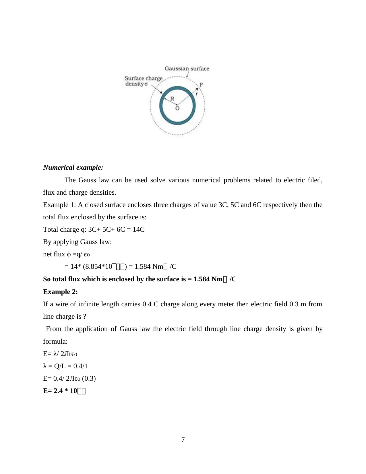
(Source: Applications of Gauss’s Law, 2019)
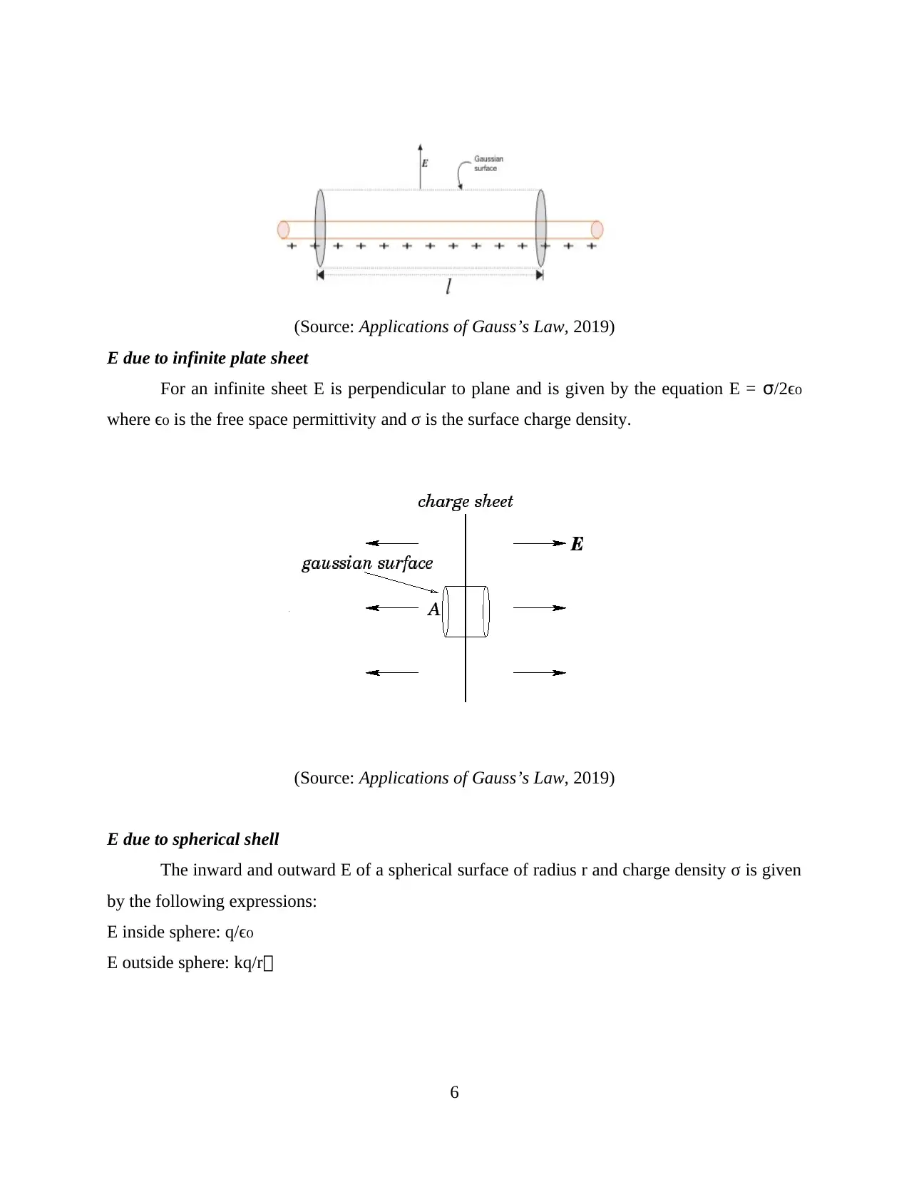
E due to infinite plate sheet
For an infinite sheet E is perpendicular to plane and is given by the equation E = σ/2ϵ₀
where ϵ is the free space permittivity and σ is the surface charge density.₀
(Source: Applications of Gauss’s Law, 2019)
E due to spherical shell
The inward and outward E of a spherical surface of radius r and charge density σ is given
by the following expressions:
E inside sphere: q/ϵ₀
E outside sphere: kq/r
6
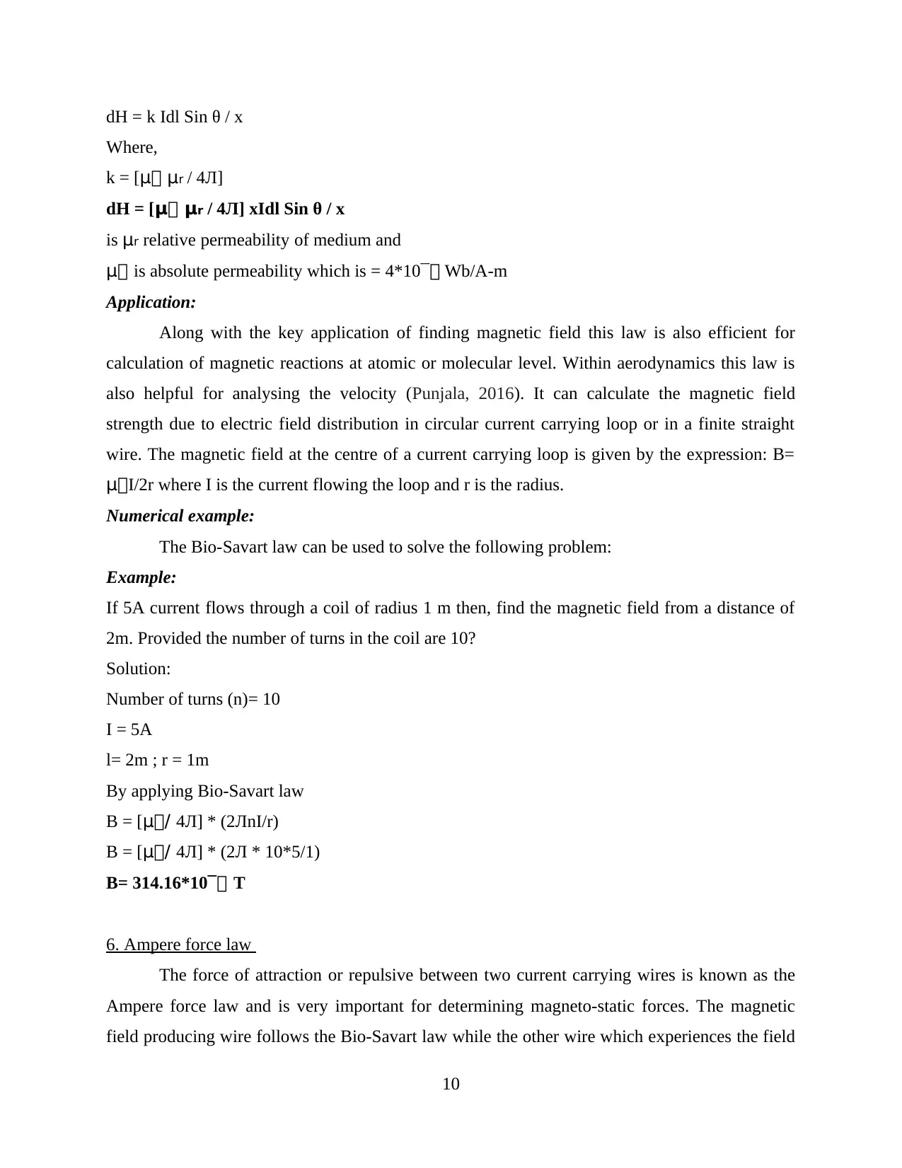
Numerical example:
The Gauss law can be used solve various numerical problems related to electric filed,
flux and charge densities.
Example 1: A closed surface encloses three charges of value 3C, 5C and 6C respectively then the
total flux enclosed by the surface is:
Total charge q: 3C+ 5C+ 6C = 14C
By applying Gauss law:
net flux ϕ =q/ ϵ₀
= 14* (8.854*10¯) = 1.584 Nm /C
So total flux which is enclosed by the surface is = 1.584 Nm /C
Example 2:
If a wire of infinite length carries 0.4 C charge along every meter then electric field 0.3 m from
line charge is ?
From the application of Gauss law the electric field through line charge density is given by
formula:
E= λ/ 2Лrϵ₀
λ = Q/L = 0.4/1
E= 0.4/ 2Лϵ (0.3)₀
E= 2.4 * 10
7
⊘ This is a preview!⊘
Do you want full access?
Subscribe today to unlock all pages.
Trusted by 1+ million students worldwide
4. Permanent and electromagnets
Permanent magnets:
This type of magnet is capable of producing persistent magnetic field at its own due to
magnetised characteristics of its constituent material. Thus, its magnetic characteristics are
permanent and depends upon the material utilised for its fabrication. One of the disadvantage of
permanent magnet is that with time their strength is reduced and their poles are constant.
Permanent magnets produces magnetic fields at lower temperature thus it is not suitable for the
applications which are based upon high temperature (Weber and et.al., 2018). The magnetic
properties of permanent magnet can be regained or recovered only with the help of re-
magnetizing process. However contrary to the electromagnets it does not require regular
electrical supply to sustain its magnetic properties.
Electromagnets:
In electromagnets magnetic fields are produced by the electric current and thus its
strength can vary and depends upon the current flow (Krishnan, 2016). Electromagnets are made
up of coil which shows magnetic behaviour when current flows through it. Usually it is wrapped
with a ferromagnetic material so that its magnetic strength can be increased. This type of
materials are also able to hold and attract the ferrous materials.
Comparison:
One of the advantage of electromagnets is that they allow the controlled power handling.
Thus, the power can be released or hold as per the needs. It makes them highly suitable for the
applications based upon DC current. Both types of the discussed magnets possess magnetism
properties and have imaginary magnetic field lines. Though electromagnets have certain
advantages over permanent one such as variable magnetic strength and low cost but it also has
certain disadvantages. The key disadvantage of electromagnets is that continuous electric supply
leads to ohmic heating, core losses and voltage spikes which are not desirable. It is also observed
that as electromagnets require copper coupling in greater number so they cannot be used in small
space and is less feasible for maintaining and repairing in case of damage.
Applications:
Permanent magnets are used for converting electricity into mechanical forces, electric
motors, measuring instruments, trains, myriad applications, magnetic levitation and in generators
(Härtel, 2018). On the other hand electromagnets are primarily used in electrical transformers
8
Paraphrase This Document
Need a fresh take? Get an instant paraphrase of this document with our AI Paraphraser
and other electric devices. The solar power applications and the machines which needs minimum
copper losses also employs permanent magnet. The versatility and strength of electromagnets
makes them suitable for industrial applications and in variety of electric devices such as lifting
magnets, relays, motors, data storage equipments, transformers loudspeakers and magnetic locks.
5. Bio- Savart law
Bio-Savart law is defined as the equation which describes the magnetic fields produced
due to a current carrying conductor or wire so that its strength can be determined at various
points. Thus, it describes the current as the source of magnetic field when the distance between
current source and field point is continuously changing (Greaves and et.al., 2018).
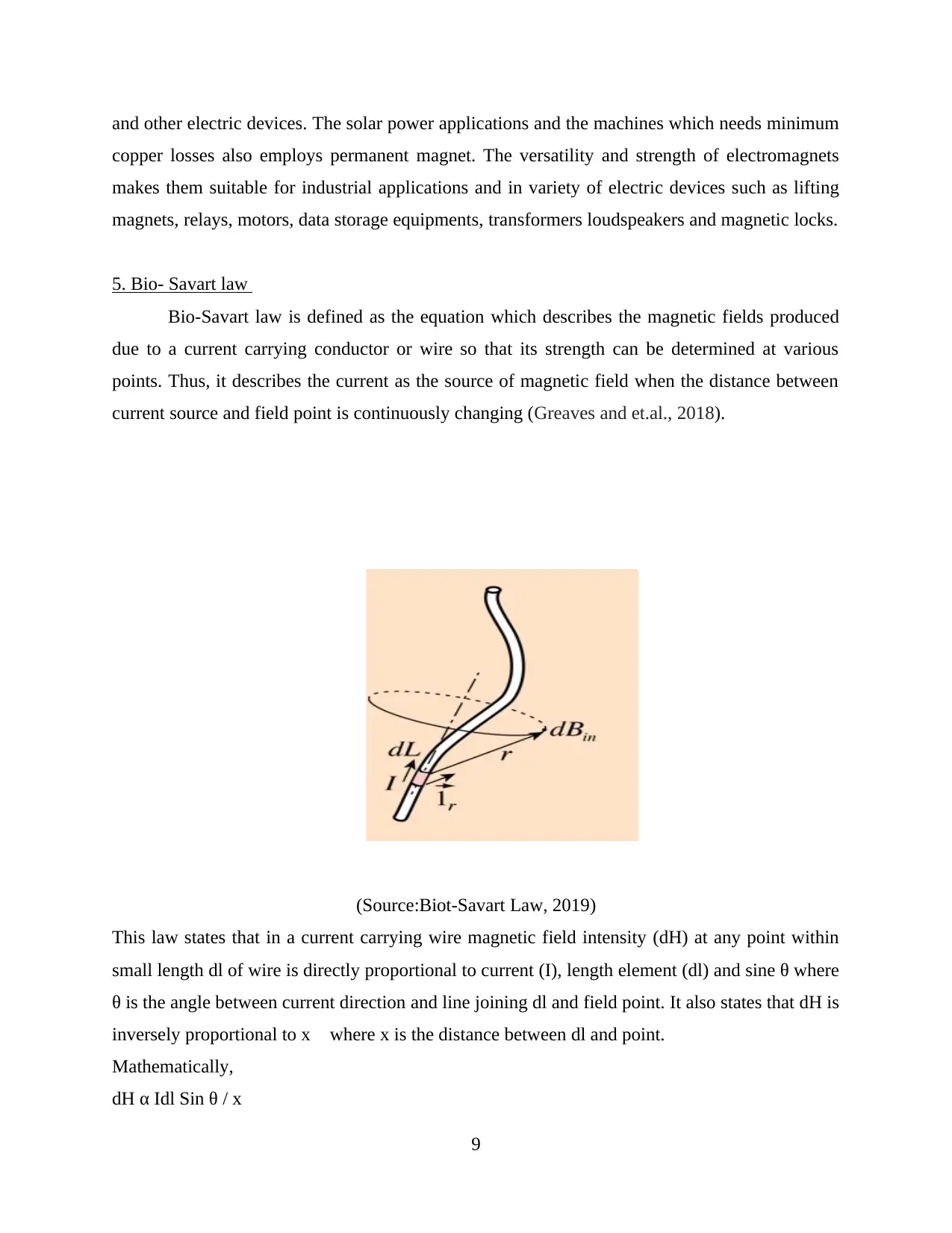
(Source:Biot-Savart Law, 2019)
This law states that in a current carrying wire magnetic field intensity (dH) at any point within
small length dl of wire is directly proportional to current (I), length element (dl) and sine θ where
θ is the angle between current direction and line joining dl and field point. It also states that dH is
inversely proportional to x where x is the distance between dl and point.
Mathematically,
dH α Idl Sin θ / x
9
copper losses also employs permanent magnet. The versatility and strength of electromagnets
makes them suitable for industrial applications and in variety of electric devices such as lifting
magnets, relays, motors, data storage equipments, transformers loudspeakers and magnetic locks.
5. Bio- Savart law
Bio-Savart law is defined as the equation which describes the magnetic fields produced
due to a current carrying conductor or wire so that its strength can be determined at various
points. Thus, it describes the current as the source of magnetic field when the distance between
current source and field point is continuously changing (Greaves and et.al., 2018).
(Source:Biot-Savart Law, 2019)
This law states that in a current carrying wire magnetic field intensity (dH) at any point within
small length dl of wire is directly proportional to current (I), length element (dl) and sine θ where
θ is the angle between current direction and line joining dl and field point. It also states that dH is
inversely proportional to x where x is the distance between dl and point.
Mathematically,
dH α Idl Sin θ / x
9
dH = k Idl Sin θ / x
Where,
k = [μ μr / 4Л]
dH = [μ μr / 4Л] xIdl Sin θ / x
is μr relative permeability of medium and
μ is absolute permeability which is = 4*10¯ Wb/A-m
Application:
Along with the key application of finding magnetic field this law is also efficient for
calculation of magnetic reactions at atomic or molecular level. Within aerodynamics this law is
also helpful for analysing the velocity (Punjala, 2016). It can calculate the magnetic field
strength due to electric field distribution in circular current carrying loop or in a finite straight
wire. The magnetic field at the centre of a current carrying loop is given by the expression: B=
μI/2r where I is the current flowing the loop and r is the radius.
Numerical example:
The Bio-Savart law can be used to solve the following problem:
Example:
If 5A current flows through a coil of radius 1 m then, find the magnetic field from a distance of
2m. Provided the number of turns in the coil are 10?
Solution:
Number of turns (n)= 10
I = 5A
l= 2m ; r = 1m
By applying Bio-Savart law
B = [μ/ 4Л] * (2ЛnI/r)
B = [μ/ 4Л] * (2Л * 10*5/1)
B= 314.16*10¯ T
6. Ampere force law
The force of attraction or repulsive between two current carrying wires is known as the
Ampere force law and is very important for determining magneto-static forces. The magnetic
field producing wire follows the Bio-Savart law while the other wire which experiences the field
10
⊘ This is a preview!⊘
Do you want full access?
Subscribe today to unlock all pages.
Trusted by 1+ million students worldwide
1 out of 17
Related Documents


Your All-in-One AI-Powered Toolkit for Academic Success.
+13062052269
info@desklib.com
Available 24*7 on WhatsApp / Email
![[object Object]](/_next/static/media/star-bottom.7253800d.svg)
Unlock your academic potential
Copyright © 2020–2026 A2Z Services. All Rights Reserved. Developed and managed by ZUCOL.