Analysis of Factors Impacting Employee Weekly Income

This report presents an analysis of the factors influencing employee weekly income, based on an online survey of 100 individuals. The study employs LASSO and LAR models to identify significant variables. The analysis reveals that age, sex, qualification, and time spent working are correlated with income, while ethnicity shows no significant association. The report includes descriptive statistics on population characteristics like age, sex, and ethnicity, along with correlation analysis and regression model results. The findings suggest that highly skilled, experienced employees, working longer hours, and focusing on employing more men can positively impact weekly income. The study concludes with limitations, recommendations, and references to support the findings.

FACTORS AFFECTING EMPLOYEE INCOME
1

Table of Contents
1. Introduction.................................................................................................................................4
1.1. Problem statement.................................................................................................................5
1.2. Research questions.................................................................................................................5
1.3. Research objective.................................................................................................................6
1.4. Specific objectives.................................................................................................................6
2.0. Data................................................................................................................................................6
2.1. Online survey..............................................................................................................................6
2.2. Data description..........................................................................................................................6
3.0. Data analysis............................................................................................................................7
3.1. LASSO (Least Absolute Shrinkage and Selection Operator)..................................................7
3.2. LAR (Least Angle Regression)...............................................................................................7
3.3. Hypotheses............................................................................................................................8
3.4. Results...................................................................................................................................8
3.5. Population characteristics.....................................................................................................8
3.5.1. Age.................................................................................................................................8
Table 1...............................................................................................................................................9
Age Frequency Table.....................................................................................................................9
3.5.2. Sex.................................................................................................................................9
Table 2...............................................................................................................................................9
3.5.3. Age and sex..................................................................................................................10
Table 3.............................................................................................................................................10
3.5.4. Ethnicity.......................................................................................................................11
Table 4.............................................................................................................................................11
Bar Chart 1......................................................................................................................................11
3.6. Inferential statistics.............................................................................................................12
3.6.1. Correlation analysis.....................................................................................................12
Table 5.............................................................................................................................................13
3.6.2. Model 4 LAR and LASSO.............................................................................................13
Table 6.............................................................................................................................................14
Table 7.............................................................................................................................................15
Table 8.............................................................................................................................................15
Table 9.............................................................................................................................................15
Histogram Chart 1...............................................................................................................................16
3.7. Discussion............................................................................................................................16
4.0. Conclusion..............................................................................................................................18
2

5.0. Limitation...................................................................................................................................19
6.0. Recommendation........................................................................................................................19
References...........................................................................................................................................20
7.0. Appendix......................................................................................................................................21
Appendix A..........................................................................................................................................21
Appendix B.........................................................................................................................................22
Appendix C.........................................................................................................................................23
Appendix D: Data................................................................................................................................24
3

Executive summary
Every individual and companies transact businesses with the aim to generate income as well
as earning for a living. Employees get salaries as compensation of their labor or services they
provide. Age, sex, gender, qualification, ethnicity and time spent in doing work are
independent factors that affect dependent factor which is weekly income. However, these
variables were selected by use of LASSO (Least Absolute Shrinkage and Selection Operator)
and LAR (Least Angle Regression) model selection to find the best factors to be fit in a
regression model. Four variables that are age, sex, qualification and time in hours, were
positively correlated with the dependent variable (weekly income). Except for ethnicity
whose p-value is greater than 0.05, four variables that are age, sex, qualification and time
spent in work were statistically significant with their p value<0.05. Individuals and
companies should, therefore, hire highly skilled personnel with high qualification,
experienced employees, increase time spent in working and focus on employing more men
than women; this will make a great impact on the weekly income.
1. Introduction
Income is the revenue generated from selling goods and services (Haraldsson, 2017).
(DAVID, 2011) Define it as the money that an individual receives in compensation for his or
her labor and services. (Jones, 2010) Studies on the factors that affect income reveal that
qualification is a measure of one’s potentiality and therefore, highly skilled personnel tend to
generate more income in both the private and public sector. Another study conducted in New
Zealand reveals that qualification is directly proportional to income (Sheree, 2012) whereby
the greater the level of qualification the higher the income. The time that individuals spent in
doing work have a great influence on the weekly income as revealed by (Asafa, 2015).
However, studies by (Volkoff, 2010) indicate that older people tend to spend less time in
work because of their vulnerability based on depression, tiresome, and memory capacity to
4

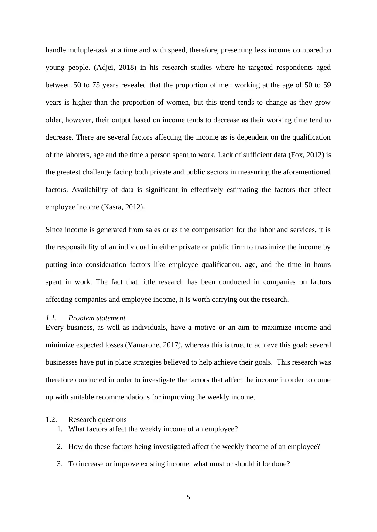
handle multiple-task at a time and with speed, therefore, presenting less income compared to
young people. (Adjei, 2018) in his research studies where he targeted respondents aged
between 50 to 75 years revealed that the proportion of men working at the age of 50 to 59
years is higher than the proportion of women, but this trend tends to change as they grow
older, however, their output based on income tends to decrease as their working time tend to
decrease. There are several factors affecting the income as is dependent on the qualification
of the laborers, age and the time a person spent to work. Lack of sufficient data (Fox, 2012) is
the greatest challenge facing both private and public sectors in measuring the aforementioned
factors. Availability of data is significant in effectively estimating the factors that affect
employee income (Kasra, 2012).
Since income is generated from sales or as the compensation for the labor and services, it is
the responsibility of an individual in either private or public firm to maximize the income by
putting into consideration factors like employee qualification, age, and the time in hours
spent in work. The fact that little research has been conducted in companies on factors
affecting companies and employee income, it is worth carrying out the research.
1.1. Problem statement
Every business, as well as individuals, have a motive or an aim to maximize income and
minimize expected losses (Yamarone, 2017), whereas this is true, to achieve this goal; several
businesses have put in place strategies believed to help achieve their goals. This research was
therefore conducted in order to investigate the factors that affect the income in order to come
up with suitable recommendations for improving the weekly income.
1.2. Research questions
1. What factors affect the weekly income of an employee?
2. How do these factors being investigated affect the weekly income of an employee?
3. To increase or improve existing income, what must or should it be done?
5

1.3. Research objective
The general objective of this study is to determine the factors that affect employee weekly
income.
1.4. Specific objectives
1. To investigate if there is a linear relationship between the time spent on work and the
weekly income.
2. To identify the effect of the qualification on employee weekly income.
3. To identify the effect of age on employee weekly income.
4. To investigate how gender and ethnicity affect employee weekly income
2.0. Data
2.1. Online survey
A survey refers to the process of data collection on various aspects or characteristics of a
study population. This research will make use of an online survey data that was presented in
form of questionnaires and administered online to the target population. The respondents
received the questionnaires via their emails, filled and returned them.
An online survey is the most effective method of data collection for this research as it allows
for freedom of filling the questions at respondents’ own pleasure and also it is less cost
effective.
2.2. Data description
Both primary and secondary sources of data collected were used in this research. An online
survey was employed for collecting primary data while company websites
http://new.censusatstudent.org.nz/resource/nz-incomes-surf/ was used for collecting
secondary data. The sample size is 100 individuals consisting of both male and female that
was obtained through random sampling. In addition, the targeted respondents are aged
between 25 to 64 years. The data variables are age, sex, ethnicity, qualification, and income.
6

3.0. Data analysis
3.1. LASSO (Least Absolute Shrinkage and Selection Operator)
LASSO is a shrinkage and variable selection method for linear models. It is a regression
analysis technique that performs both variable determination and regularization so as to
improve the forecast exactness and interpretability of the factual model it produces. It is an
extension of linear regression using shrinkage.
A Stepwise method was used for selecting the best model. This is a method of fitting
regression models in which the choice of predictive variables is carried out by an automatic
procedure. In each step, a variable is considered for addition to or subtraction from the set of
explanatory variables based on some predetermined criterion.
The method shall select variables to be included in the model one after another.
Model 1: income = age
Model 2: income = age + sex
Model 3: income = age + sex + qualification
Model 4: income = age + sex + qualification + time in hours
Model 4 is the best lasso model as it includes only the variables that are statistically
significant.
3.2. LAR (Least Angle Regression)
LAR is a technique of fitting a regression model for a linear combination of a subset of
potential covariates. The calculation is like forward stepwise regression, however as opposed
to including factors at each progression, the evaluated parameters are increased toward a path
equiangular to everyone's relationships with the residual.
7

To select the best method, we use forward regression. This is a technique which involves
starting with no variables in the model, testing the addition of each variable using a chosen
model fit criterion. We found that the model below is fit for this study.
Income = age + sex + qualification+ time in hours
3.3. Hypotheses
Given the models selected from lasso and LAR, we shall investigate the following
hypotheses;
i. H0: Age does not affect employee weekly income.
H1: Age does affect employee weekly income.
ii. H0: Sex does not affect employee weekly income
H1: Sex does affect employee weekly income
iii. H0: Qualification does not affect employee weekly income
H1: Qualification does affect employee weekly income
iv. H0: Time in hours does not affect weekly employee income.
H1: Time in hours does not affect weekly employee income.
3.4. Results
Based on the two information criterion lasso and LAR, we shall investigate the factors that
affect the income. The following variables shall be examined on their effect on income; age,
sex, qualification, and time in hours that an employee or individuals spent working in a week.
3.5. Population characteristics
3.5.1. Age
The population was aged between 25 to 60 years of age. Most population 23 representing
23% were aged between 30-34 years followed by 19 representing 19% who were aged
between 25 to 29 years. The lowest number of respondents 7(7%) of respondents from the
data were aged between 60 to 64 years.
8

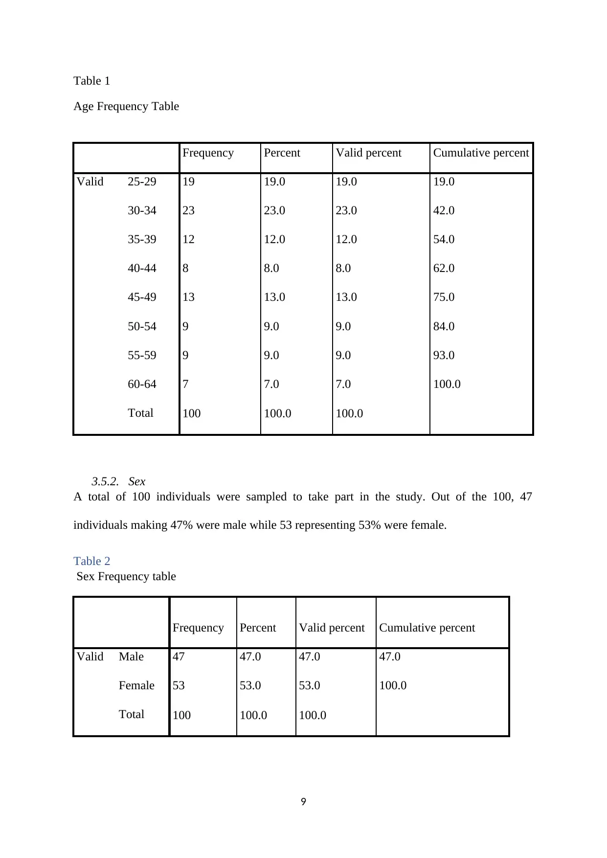
Table 1
Age Frequency Table
Frequency Percent Valid percent Cumulative percent
Valid 25-29 19 19.0 19.0 19.0
30-34 23 23.0 23.0 42.0
35-39 12 12.0 12.0 54.0
40-44 8 8.0 8.0 62.0
45-49 13 13.0 13.0 75.0
50-54 9 9.0 9.0 84.0
55-59 9 9.0 9.0 93.0
60-64 7 7.0 7.0 100.0
Total 100 100.0 100.0
3.5.2. Sex
A total of 100 individuals were sampled to take part in the study. Out of the 100, 47
individuals making 47% were male while 53 representing 53% were female.
Table 2
Sex Frequency table
Frequency Percent Valid percent Cumulative percent
Valid Male 47 47.0 47.0 47.0
Female 53 53.0 53.0 100.0
Total 100 100.0 100.0
9

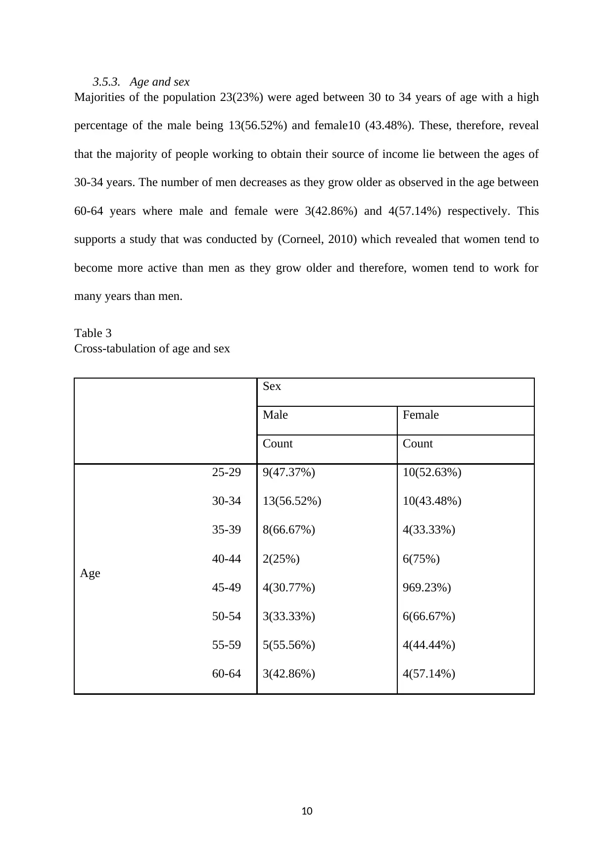
3.5.3. Age and sex
Majorities of the population 23(23%) were aged between 30 to 34 years of age with a high
percentage of the male being 13(56.52%) and female10 (43.48%). These, therefore, reveal
that the majority of people working to obtain their source of income lie between the ages of
30-34 years. The number of men decreases as they grow older as observed in the age between
60-64 years where male and female were 3(42.86%) and 4(57.14%) respectively. This
supports a study that was conducted by (Corneel, 2010) which revealed that women tend to
become more active than men as they grow older and therefore, women tend to work for
many years than men.
Table 3
Cross-tabulation of age and sex
Sex
Male Female
Count Count
Age
25-29 9(47.37%) 10(52.63%)
30-34 13(56.52%) 10(43.48%)
35-39 8(66.67%) 4(33.33%)
40-44 2(25%) 6(75%)
45-49 4(30.77%) 969.23%)
50-54 3(33.33%) 6(66.67%)
55-59 5(55.56%) 4(44.44%)
60-64 3(42.86%) 4(57.14%)
10

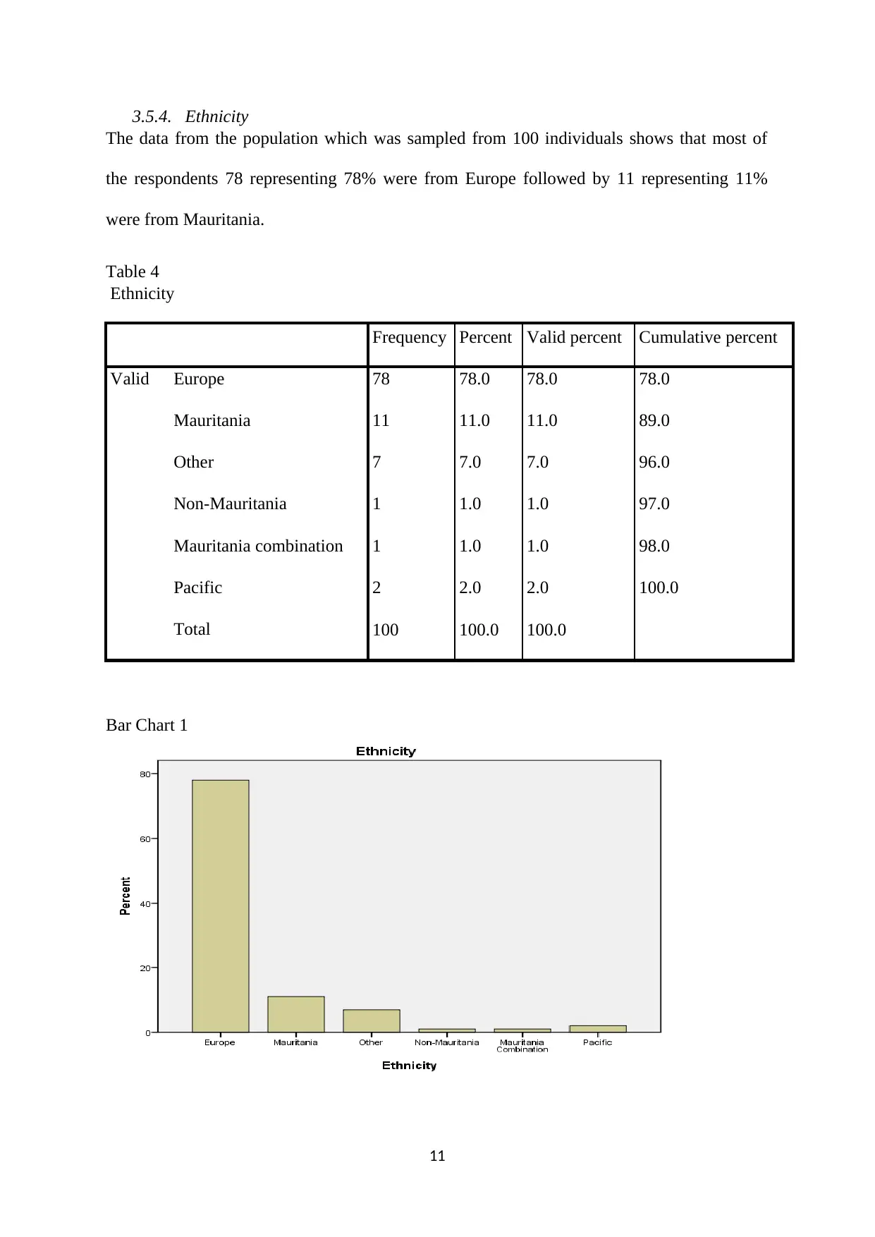
3.5.4. Ethnicity
The data from the population which was sampled from 100 individuals shows that most of
the respondents 78 representing 78% were from Europe followed by 11 representing 11%
were from Mauritania.
Table 4
Ethnicity
Frequency Percent Valid percent Cumulative percent
Valid Europe 78 78.0 78.0 78.0
Mauritania 11 11.0 11.0 89.0
Other 7 7.0 7.0 96.0
Non-Mauritania 1 1.0 1.0 97.0
Mauritania combination 1 1.0 1.0 98.0
Pacific 2 2.0 2.0 100.0
Total 100 100.0 100.0
Bar Chart 1
11

3.6. Inferential statistics
3.6.1. Correlation analysis
Correlation analysis is carried out to assess the relationship between variables. Of more
interest in this analysis, is the correlation between the dependent and independent variables
Results depict that ethnicity does not show any significant association with the dependent
variable, income since its p-values exceed the critical value, 0.05. The variables age, sex,
qualification and hours spent in work depict a statistically significant relationship between
them and the dependent variable, income.
The Pearson correlation coefficient between sex and income is -0.391 implying a negative
association between the two variables. A change in sex in one direction results to a change in
the income in the opposite direction.
The Pearson correlation coefficient between age and income was found to be 0.122 implying
that there exists a positive association between age and income. This positive association can
be interpreted as; an increase in age by one-year results to a corresponding increase in income
by about 0.122 units. This can be attributed to experience gained in particular work as time
goes by.
The Pearson correlation coefficient between qualification and income was found to be 0.198
implying a positive association between employee qualification and income generated. The
0.198 association coefficient can be interpreted as; an increase in the number of qualified
employees by one result to a corresponding increase in income by about 0.198 units.
The Pearson correlation coefficient between time in hours and weekly income was found to
be 0.405 implying a positive association between time and income generated. The 0.405
association coefficient can be interpreted as; an increase of time by one-unit results to
corresponding increases in income by about 0.405 units.
12

Table 5
Correlations
Income Age Sex Ethnicity Qualification Hours
Pearson
correlation
Income 1.000 .122 -.391 -.074 .198 .405
Age .122 1.000 .092 .132 -.216 .081
Sex -.391 .092 1.000 -.107 -.177 -.407
Ethnicity -.074 .132 -.107 1.000 -.090 .101
Qualification .198 -.216 -.177 -.090 1.000 -.088
Hours .405 .081 -.407 .101 -.088 1.000
Sig. (1-tailed) Income . .113 .000 .231 .024 .000
Age .113 . .181 .096 .015 .212
Sex .000 .181 . .144 .039 .000
Ethnicity .231 .096 .144 . .186 .159
Qualification .024 .015 .039 .186 . .191
Hours .000 .212 .000 .159 .191 .
N Income 100 100 100 100 100 100
Age 100 100 100 100 100 100
Sex 100 100 100 100 100 100
Ethnicity 100 100 100 100 100 100
Qualification 100 100 100 100 100 100
Hours 100 100 100 100 100 100
**. Correlation is significant at the 0.01 level (1-tailed).
*. Correlation is significant at the 0.05 level (1-tailed).
3.6.2. Model 4 LAR and LASSO
We examined the following model and its variables.
13

Income = Age + Sex + Qualification+ Time in hours
Except for ethnicity, the independent variables age, sex, qualification, and time in hours were
found to be statistically significantly associated with income. This is because the p-values for
the association between the variables were less than 0.05 implying a rejection of the null
hypothesis that there is no association between the dependent and independent variables.
Age, qualification, and time in hours depict a positive association with the dependent variable
while sex was negatively associated with income
Table 6
Correlations
Income Age Sex Qualification Hours
Pearson correlation Income 1.000 .122 -.391 .198 .405
Age .122 1.000 .092 -.216 .081
Sex -.391 .092 1.000 -.177 -.407
Qualification .198 -.216 -.177 1.000 -.088
Hours .405 .081 -.407 -.088 1.000
Sig. (1-tailed) Income . .113 .000 .024 .000
Age .113 . .181 .015 .212
Sex .000 .181 . .039 .000
Qualification .024 .015 .039 . .191
Hours .000 .212 .000 .191 .
N Income 100 100 100 100 100
Age 100 100 100 100 100
Sex 100 100 100 100 100
Qualification 100 100 100 100 100
Hours 100 100 100 100 100
*. Correlation is significant at the 0.05 level (1-tailed).
**. Correlation is significant at the 0.01 level (1-tailed).
14

Regression analysis was conducted including all the variables involved in model 4 LAR and
LASSO.
Table 7
Model summary
Model R R square
Adjusted r
square
Std. Error of the
estimate
1 .550a .303 .266 403.65438
A. Predictors: (constant), hours, age, ethnicity, qualification, sex
R square equals 0.303 implying that the independent variables explain about 30.3% of the
dependent variable.
Table 8
ANOVAa
Model Sum of squares Df Mean square F Sig.
1 Regression 6659306.192 5 1331861.238 8.174 .000b
Residual 15316064.808 94 162936.860
Total 21975371.000 99
A. Dependent variable: income
B. Predictors: (constant), hours, age, ethnicity, qualification, sex
ANOVA regression test had a p-value of 0.000 implying that it would be statistically
significant to include an ANOVA model.
Table 9
Coefficientsa
Model
Unstandardized coefficients Standardized coefficients
T Sig.B Std. Error Beta
1 (constant) 415.244 276.672 1.501 .137
Age 38.084 18.584 .183 2.049 .043
15

Sex -241.105 92.017 -.257 -2.620 .010
Ethnicity -66.542 41.964 -.139 -1.586 .116
Qualification 80.130 34.956 .208 2.292 .024
Hours 10.172 3.084 .318 3.298 .001
A. Dependent variable: income
Histogram Chart 1
The independent variable to be included in the prediction model include age, sex,
qualification, and time(hours) since their p-values are less than 0.05 implying that they would
be statistically significant in the model.
Our regression model shall therefore be;
Income=415.244+ 38.084∗AGE−241.105∗SEX +80.130∗Qualification+10.172∗time ¿)
3.7. Discussion
Results of the analysis have shown that several factors affect weekly income. The factors are
as discussed below;
i. Age
16

Results of the regression analysis show that age explains about 38.084 times of the
dependent variable (income). The more an individual grows older, the more experience
one gain and subsequently more income generated (Burns, 2015).
However, in his study on the active population between young and old adult, a conflicting
result was obtained by (Zell, 2014). He failed to find any statistical association age and
income.
ii. Sex
Results of the regression analysis depict the negative effect of sex on plasma beta-
carotene with a coefficient of - 241.105. This is an implication that a change in gender
would result in a change in income in the opposite direction by about 241.105 units.
Since the female gender is represented by a higher number compared to the male gender,
it would be right to argue that the female gender shall have a negative impact on income.
Similar findings have been found by previous researchers, including (Lo Sasso, 2011) and
(Sueuk, 2016) they both argued that women were negatively associated with income.
Contradicting results were obtained by (Stoet, 2013) found out that there exists no
association between sex and income. These results were almost similar to those observed
by (Vandelanotte, 2010). Vandelanotte observed an association coefficient of -0.003
between gender and income.
iii. Qualification
The findings have depicted high qualification has positive impacts on income with a
regression coefficient of 80.130. This implies that an increase employee with high
qualification leads to an increase in income. Qualification explains about 80.13 times of
the dependent variable. (Olckers, 2015) Studies reveal that the highly skilled personnel
17

tend to produce a better result and subsequently better income; which agrees with
findings of the current study.
iv. Time(hours)
The study found out a positive relationship between time in hours and weekly income
with a regression coefficient in 10.172. This implies that an increase in time that
employees work by 1 hour would lead to an increase in weekly income by 10.172 units.
Consequentially, a decrease in time that employees work by 1 hour would result in 10.172
units decrease in weekly income. Our current findings are similar to the findings of
(Kolodziejczyk, 2012)
Contradicting findings have previously been shown by (Jarousse, 2010) who failed to find
any significant relationship between the two variables. He found a significant value of
0.63 which is greater than the critical point 0.05. He concluded that working less time
and increase earning.
4.0. Conclusion
Factor selection is crucial and challenging in this field of study, mainly because the desired
output varies for a different set of data, and it is hard to find a model that works for every
kind of problem. For these reasons, the present study made use of the LAR model selection
techniques. The techniques helped us to identify the model with the most relevant features
(variables) for the dataset to analyze. The task becomes even more challenging when dealing
with high-dimensional datasets.
The findings of the present study have shown that a number of factors affect weekly income.
Among these factors are age, sex, employee qualification, and time in hours that an
individual spent in working. These factors have a different impact on the dependent variable
(weekly income). High qualification, time in hours and age were found to positively affect
18

employee weekly income whereas sex had a negative impact on employee weekly income.
Proper control measures should, therefore, be taken to control for these factors in order for
companies and individuals to increase their weekly income.
5.0. Limitation
Apart from the independent variables being investigated in this research, there are other
factors which involve managerial and political factors which affect the dependent variable
income and was not discussed in this research. Furthermore, there is little research that has
been conducted relating factors affecting employee income.
6.0. Recommendation
From the results of the analysis of this research, the following are the recommendation which
should be employed to increase the income by the employees or companies both public and
private
i. Employers should put qualification into consideration during employment as this
factor correlate positively with income.
ii. Ethnicity is not a factor to consider during employment at all. This variable is not
statistically significant rendering it unnecessary.
iii. Employees and individuals from both the public and private sector should increase
their time to work to increase their weekly income. Time spent in a week to work is
positively correlated to weekly income,
iv. Age is a factor which is positively correlated with income. This is due to experience
gained every year by the employee. Experienced employees should be given priorities
for employment than inexperienced people in order to increase weekly income
19

References
Adjei, N. K. (2018). The Capability of multi-tasking among the age population. International Journal
for Equity in Health, 2-12.
Asafa Jalata, H. F. (2015). Current Perspectives in Social Theory. Capitalism and the Common Sense
of Time and Money, 29-74.
Burns, W. (2015). Textile-Led Design for the Active Ageing Population. Experiences in the design,
iterative development, and evaluation of a technology-enabled garment for active ageing
Vandelanotte, M. J. (2010). Australian and New Zealand Journal of Public Health. Physical activity
trends in Queensland (2002 to 2008): are women becoming more active than men?, 248-254.
Current Perspectives in Social Theory. (2015). Capitalism and the Common Sense of Time and Money,
29-74.
DAVID L. SJOQUIST, A. V. (2011). Public Budgeting and Finance. The Impact of Tax Revenue from
Capital Gains Realizations on State Income Tax Revenue and Budget Conditions, 31-48.
Fox, C. K. (2012). A Lack of Strategies for Effective Decision Making. insufficient data, 33-38.
Haraldsson, M. (2017). When revenues are not revenues: the influence of municipal governance on
revenue recognition within Swedish municipal waste management. Local Government
Studies, 669-688.
Jarousse, J.-P. (2010). Economics of Education Review. Working less to earn more: An application to
the analysis of rigidity in educational choices, 50-62.
Jones, J. P. (2010). Factors Affecting Income. The Journal of Higher Education, 185-190.
Lo Sasso, A. T.-F. (2011). The Unexplained Trend Of Men Earning More Than Women. Pay Gap For
Newly Trained Physicians, 194-212.
Olckers, C. P. (2015). European J of International Management. Psychological ownership as a
requisite for talent retention: the voice of highly skilled employees, 53-59.
Volkoff, C. B. (2010). Applied economics. Does intense time pressure at work make older employees
more vulnerable? A statistical analysis based on a French survey, 754-762.
Sheree J. Gibb, D. M. (2012). Childhood family income and life outcomes in adulthood: Findings from
a 30-year longitudinal study in New Zealand. Social Science & Medicine, 8.
Stoet, G. O. (2013). Are women better than men at multi-tasking? BMC Psychology, 2-10.
Sueuk, U. P. (2016). Men earn substantially more than women. Board & Administrator for
Administrators Only, 5-9.
Yamarone, R. (2017). Maximize Profits and Minimize Losses. Journal of economic, 23-28.
20

Zell, E. B. (2014). Social Psychological and Personality Science. ou May Think You're Right, Young
Adults Are More Liberal Than They Realize, 327-338.
7.0. Appendix
Appendix A
21

Appendix B
22

Appendix C
23

Appendix D: Data
Age
midpoin
t
Age
Categor
y
Sex Ethnicity Highest
qualification
Weekly
hours
Weekly
income
27.5 25-29 Femal
e Europe Vocational
training 37 560
27.5 25-29 Male Mauritania Vocational
training 45 530
27.5 25-29 Femal
e Europe Student 29 270
27.5 25-29 Male Europe Other Post-
Secondary 43 810
27.5 25-29 Femal
e Europe Vocational
training 19 200
27.5 25-29 Male Europe Student 14 250
27.5 25-29 Femal
e Europe
Bachelor
degree and
above
37 1100
27.5 25-29 Male Europe Other Post-
Secondary 49 830
27.5 25-29 Femal
e Other Student 27 300
27.5 25-29 Male Mauritania Vocational
training 46 150
27.5 25-29 Male Europe Student 43 570
27.5 25-29 Male Europe Vocational
training 31 1260
27.5 25-29 Femal
e Other Student 23 470
27.5 25-29 Femal
e Europe Vocational
training 10 400
27.5 25-29 Femal
e Europe Vocational
training 14 160
27.5 25-29 Femal
e Europe Other Post-
Secondary 30 400
27.5 25-29 Male Other Vocational
training 26 620
27.5 25-29 Male Europe Vocational
training 45 750
27.5 25-29 Femal
e Europe
Bachelor
degree and
above
24 500
32.5 30-34 Male Europe Student 23 520
32.5 30-34 Male Europe Vocational
training 40 960
32.5 30-34 Femal
e Europe Vocational
training 9 480
32.5 30-34 Male Europe Student 40 1220
24

32.5 30-34 Male Europe Vocational
training 40 1490
32.5 30-34 Femal
e Europe Vocational
training 7 430
32.5 30-34 Male Europe Bachelor
degree and
above
38 880
32.5 30-34 Male Other Student 25 420
32.5 30-34 Femal
e Mauritania Vocational
training 14 330
32.5 30-34 Male Europe Bachelor
degree and
above
40 600
32.5 30-34 Femal
e Europe Student 8 120
32.5 30-34 Femal
e Europe Student 35 360
32.5 30-34 Femal
e Mauritania No
qualification 18 270
32.5 30-34 Male Europe Vocational
training 43 1040
32.5 30-34 Male Europe Bachelor
degree and
above
45 1170
32.5 30-34 Male Europe Bachelor
degree and
above
40 780
32.5 30-34 Femal
e Europe Vocational
training 40 880
32.5 30-34 Femal
e Europe Student 40 790
32.5 30-34 Femal
e Europe Vocational
training 24 600
32.5 30-34 Male Europe Other Post-
Secondary 44 980
32.5 30-34 Male Europe Other Post-
Secondary 56 750
32.5 30-34 Male Europe Vocational
training 64 750
32.5 30-34 Femal
e Europe Student 37 450
37.5 35-39 Femal
e Europe Student 38 530
37.5 35-39 Male Europe Vocational
training 45 680
37.5 35-39 Femal
e
Non-Mauritania
combination
Vocational
training 10 460
37.5 35-39 Male Mauritania No 26 240
25

qualification
37.5 35-39 Male Europe Vocational
training 32 780
37.5 35-39 Male Europe Vocational
training 36 1210
37.5 35-39 Femal
e Europe Student 28 380
37.5 35-39 Male Other
Bachelor
degree and
above
56 540
37.5 35-39 Femal
e Europe Vocational
training 20 620
37.5 35-39 Male Europe Vocational
training 40 1220
37.5 35-39 Male Mauritania No
qualification 65 1320
37.5 35-39 Male Europe Vocational
training 79 650
42.5 40-44 Femal
e Europe Student 38 530
42.5 40-44 Femal
e Mauritania Student 52 850
42.5 40-44 Femal
e Europe Other Post-
Secondary 25 580
42.5 40-44 Femal
e Europe Student 27 460
42.5 40-44 Male Europe Vocational
training 48 940
42.5 40-44 Femal
e Europe Student 40 590
42.5 40-44 Male Mauritania
Bachelor
degree and
above
25 1180
42.5 40-44 Femal
e Europe Student 20 1130
47.5 45-49 Femal
e Europe Other Post-
Secondary 28 240
47.5 45-49 Femal
e Mauritania No
qualification 40 480
47.5 45-49 Male Europe Student 40 420
47.5 45-49 Male Mauritania No
qualification 40 570
47.5 45-49 Femal
e Europe Student 27 380
47.5 45-49 Femal
e Europe No
qualification 40 630
47.5 45-49 Femal
e Europe Vocational
training 38 690
26

47.5 45-49 Male Europe
Bachelor
degree and
above
50 3680
47.5 45-49 Femal
e Europe Vocational
training 30 300
47.5 45-49 Male Other Vocational
training 28 530
47.5 45-49 Femal
e Europe Vocational
training 37 390
47.5 45-49 Femal
e Europe Vocational
training 35 1040
47.5 45-49 Femal
e Europe Other Post-
Secondary 29 400
52.5 50-54 Femal
e Europe No
qualification 40 690
52.5 50-54 Femal
e Europe Vocational
training 5 190
52.5 50-54 Male Europe Vocational
training 40 620
52.5 50-54 Male Other Vocational
training 39 1280
52.5 50-54 Femal
e Mauritania Student 35 1090
52.5 50-54 Femal
e Europe No
qualification 24 170
52.5 50-54 Male Europe Vocational
training 40 890
52.5 50-54 Femal
e Europe No
qualification 22 210
52.5 50-54 Femal
e Europe No
qualification 76 960
57.5 55-59 Male Pacific No
qualification 52 640
57.5 55-59 Femal
e Europe Student 40 640
57.5 55-59 Femal
e Pacific Vocational
training 30 200
57.5 55-59 Male Europe Student 39 710
57.5 55-59 Femal
e Europe Student 38 800
57.5 55-59 Male Europe Vocational
training 40 460
57.5 55-59 Male Europe No
qualification 29 490
57.5 55-59 Male Europe Student 29 1780
57.5 55-59 Femal
e
Europe Bachelor
degree and
above
12 460
27

62.5 60-64 Male Europe Student 42 1980
62.5 60-64 Male Europe Other Post-
Secondary 8 380
62.5 60-64 Male Mauritania
Combination Student 76 1190
62.5 60-64 Femal
e Europe Vocational
training 11 360
62.5 60-64 Femal
e Europe Other Post-
Secondary 29 290
62.5 60-64 Femal
e Europe No
qualification 59 680
62.5 60-64 Femal
e Europe Vocational
training 31 1080
28