ENEC2005 Advanced Water Engineering: Pipeline & Sewer Design Report

This report details the analysis of a water distribution network and the design of a sanitary sewer system. The water distribution analysis employs the Hardy Cross method to investigate water flow in interconnected loops, ensuring the summation of head loss is near zero through iterative adjustments. The sanitary sewer design focuses on determining appropriate pipe sizes and velocities to maintain self-cleansing, considering factors like particle size, temperature, and flow properties. The report includes calculations, assumptions, and methodologies based on continuity and energy conservation principles. Desklib offers a variety of solved assignments.

Abstract
The report explains the analysis of water distribution network and sanitary sewer system. The
analysis of the water distribution while considering two interconnecting loops along the map is
demonstrated in the first section using Hardy cross method, the application of this method
involves, the investigation of the flow of water in every single pipe, and the procedure of
iteration is performed on the loops, with a specific end goal to guarantee that the summation of
the arithmetical head loss (hf ) for any shut loops to be zero, if, the pipe flow summation ought to
be equivalent the summation of flow leaving or entering the framework through every nodes. At
each iteration, sensible changes occurred at channels flows until the point that the take head loss
results to be pretty much less or settled to zero as flow line review the second segment exhibit
the usage of the sterile sewer, where the outline is done on deciding the proper size of sewer pipe
and speed, with a specific end goal to help in deciding the alter level and incline. It ought to be
noticed that there is suppositions on the span of the particles, the speed and temperature and
other basic properties that may impact the water and sewer properties.

Introduction
The reason for distribution system is to convey water to consumers with proper quality, amount
and weight. Water distribution network system is utilized to depict all facilities used to supply
water from its source to the point of use.
Quality of a water distribution network system
1. Water quality distribution system ought not get disintegrated in the dissemination
channels.
2. Water quality distribution system ought to be fit for providing water at all the planned
spots with adequate pressure head.
3. Water quality distribution system ought to be equipped for providing the imperative
measure of water amid putting out fires.
4. The design ought to be to such an extent that no consumer would be without water
supply, amid the repair of any segment of the framework.
5. All the conveyance channels ought to be ideally laid one meter away or over the sewer
lines.
6. Water quality distribution system ought to be reasonably water-tight as to keep
misfortunes because of spillage to the base
The investigation of water distribution network systems can be performed by utilizing three
techniques. These techniques, in sequential request of their application to arrange investigations
are; Hardy Cross method, Newton-Rapson method and Linear Theory method.
Hardy Cross was proposed an exact iterative framework for organize analysis. This strategy
relies upon loops framework solution conditions which are generally called the procedure for
changing heads. A while later, Cornish moreover associated the measures to nodal-head review
conditions which is known as procedure for changing streams. Both of these procedures are
accumulated under the name of Hardy Cross technique. This methodology tries to enlighten the
nonlinear conditions related with mastermind examination by making certain doubts. The higher
power correction terms can be rejected and the loops number is little for a lone loop in spite of

the way that the hidden hypothesis is poor. In any case, rejecting coterminous loop and
considering only a solitary revision condition on the double can impact the game plan and
besides number of iteration required for joining augmentations as the measure of the framework
increases.
Pipe network system analysis
The investigation strategies used on a basic introduction of pipe are consumable if the
arrangement of pipe is adequately direct in which the flow bearing in every single pipe is
distinguished unmistakably. In a more intricate framework, funnels might be participated in
interconnected circles in such ways that will make it harder for one to choose even the heading
of stream for each particular pipe. The key associations that is used so far which incorporates the
vitality and coherence conditions and the associations among stream and head loss in each
particular pipe will in any case be connected in such a framework, yet the condition of the sheer
number should be satisfied with a specific end goal to choose the whole flow conditions which
might overpower. For this specific conditions in a framework are ordinarily comprehended with
specific composed program of a PC especially thus. However, before these undertakings were by
and large open, the utilization the manual and furthermore spreadsheet procedures were made for
analyzing the framework. These strategies give a framework between to a great degree direct
issues like those analyzed above; comparably the tremendous ones can be unwound with simply
outstanding programming. These strategies, and also more mind boggling ones, empower one to
have the capacity to answer request, for example,
* For a particular arrangement plan of stream rates, what estimation of the head losse will be
resolved in each pipe in the framework?
* Will additional head be required to be provided utilizing pump for the coveted flow to be
accomplished?
* With what amount do we anticipate that the stream rates will change with in various focuses on
the framework if another pipe is presented, interfacing two detached parts, or to supplant a more
settled, littler pipe.

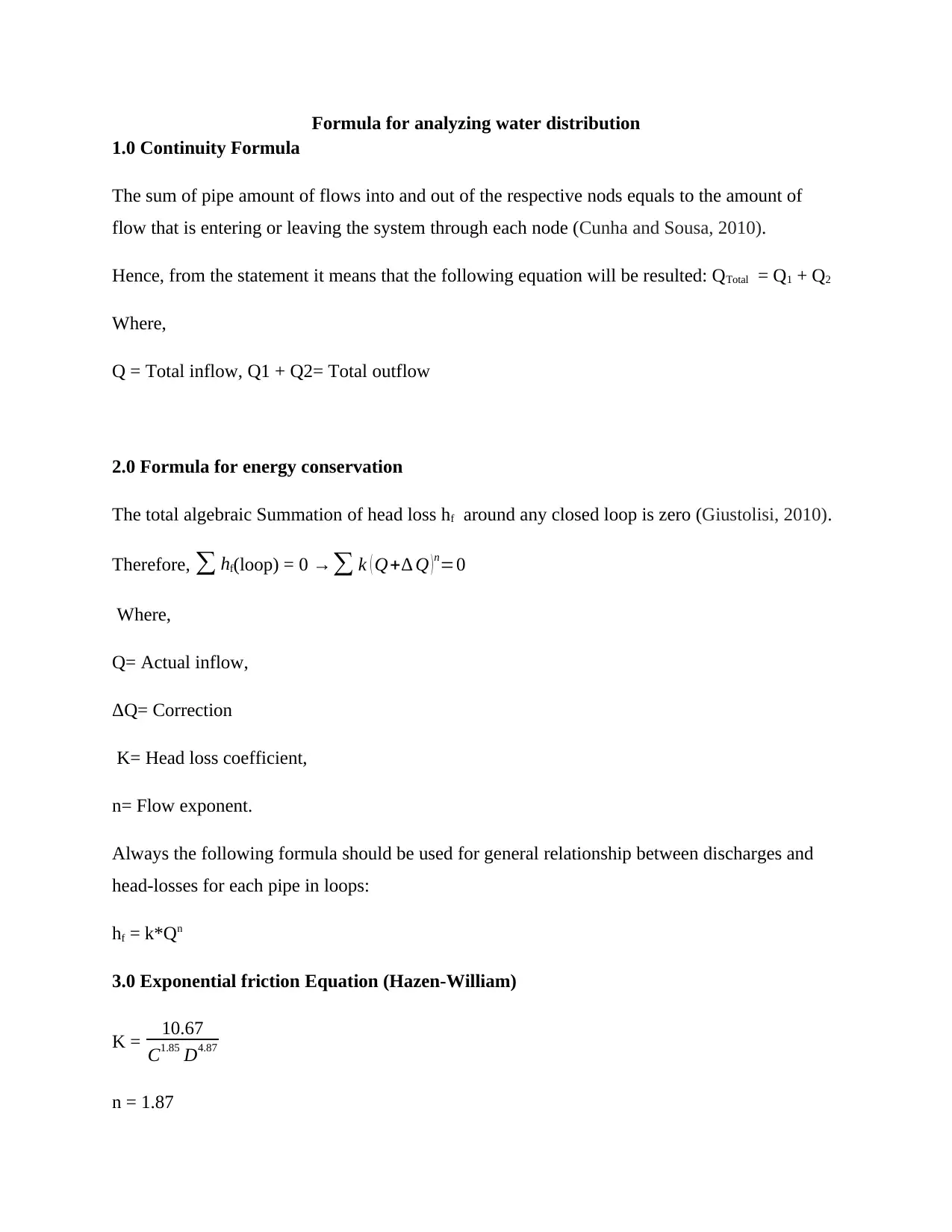
Formula for analyzing water distribution
1.0 Continuity Formula
The sum of pipe amount of flows into and out of the respective nods equals to the amount of
flow that is entering or leaving the system through each node (Cunha and Sousa, 2010).
Hence, from the statement it means that the following equation will be resulted: QTotal = Q1 + Q2
Where,
Q = Total inflow, Q1 + Q2= Total outflow
2.0 Formula for energy conservation
The total algebraic Summation of head loss hf around any closed loop is zero (Giustolisi, 2010).
Therefore, ∑ hf(loop) = 0 →∑ k ( Q+∆ Q )n=0
Where,
Q= Actual inflow,
ΔQ= Correction
K= Head loss coefficient,
n= Flow exponent.
Always the following formula should be used for general relationship between discharges and
head-losses for each pipe in loops:
hf = k*Qn
3.0 Exponential friction Equation (Hazen-William)
K = 10.67
C1.85 D4.87
n = 1.87

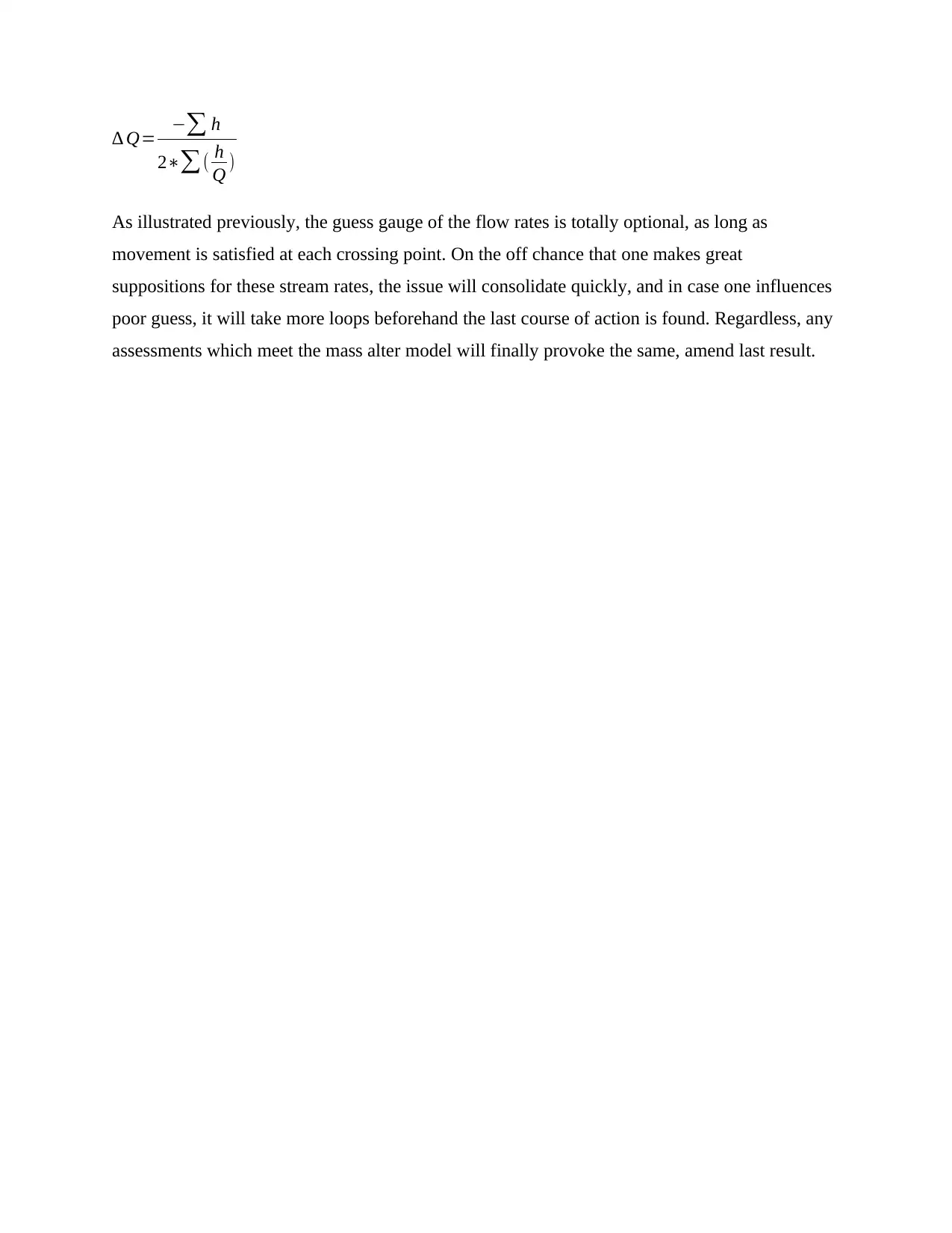
∆ Q= −∑ h
2∗∑( h
Q )
As illustrated previously, the guess gauge of the flow rates is totally optional, as long as
movement is satisfied at each crossing point. On the off chance that one makes great
suppositions for these stream rates, the issue will consolidate quickly, and in case one influences
poor guess, it will take more loops beforehand the last course of action is found. Regardless, any
assessments which meet the mass alter model will finally provoke the same, amend last result.

Methodology
Hardy cross method incorporates making a guess with respect to the flow to rate in each pipe,
taking consideration of making a guess to such an extent that the total flow into any crossing
point approaches the total flow out of that convergence. By then the head loss in each pipe is
found out, in perspective of the normal flow and the picked flow versus head loss relationship.
Next, the system is checked whether the head loss around each loop is zero. Since the
fundamental flow were speculated, this will undoubtedly not be the circumstance. The flow rates
are then adjusted with the end goal that continuity will in any case be fulfilled at each crossing
point, aside from the head loss around each loop is more similar to be zero. This strategy is
repeated until the point that the progressions are attractively little. The definite procedure is
according to the following
Procedure approach to loop
Divided the network into loops
For each loops done the fallowing steps
1. Assumptions on the flow, , flow course in the pipes, direction of flow in the loop where
positive will be taken to be clockwise or negative will be taken to be counterclockwise,
with an application of equation of continuity condition at every node. Evaluated pipe
flows are associated with iteration until head loss in the clockwise direction are
equivalent to the counterclockwise bearing in each loop.
2. The equivalent resistance K for each pipe will be required to be calculated based on the
given parameters on the demand for each node, similarly pipe length and diameter,
together with temperature and finally pipe material are expected to be unique if not it is
assumed to be equal.
3. Calculation of hf = k*𝑄n for each pipe. The sign from procedure 1 is retained and
computation is done for the sum of the loops hf

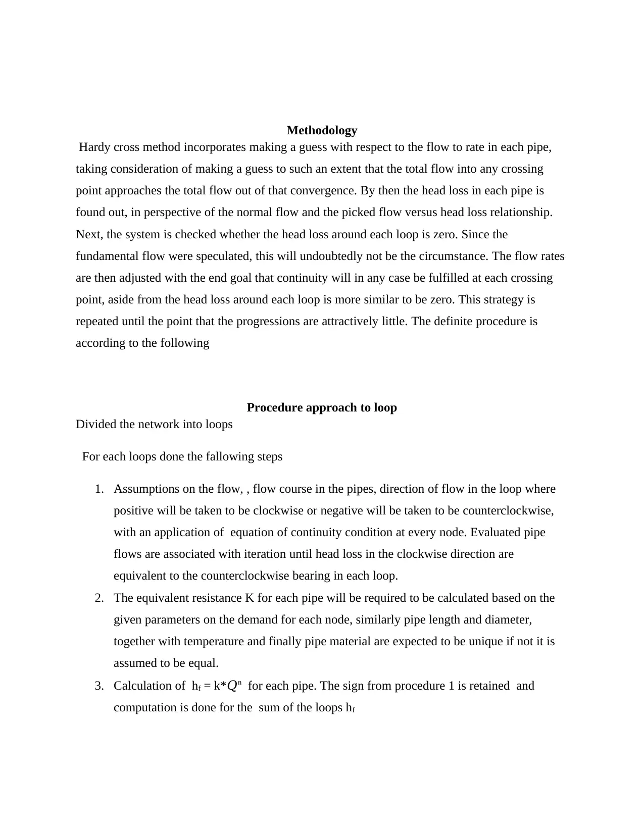
4. Computation of hf ⁄Q for each and every pipe and the summation for each and every
loop that is∑ ¿hf ⁄𝑄|.
5. Calculation of the correction by the fallowing formula ∆𝑄 = − ∑ h f/( 𝑛∑ |hf ⁄𝑄 |
6. Application of correction to Qnew = Q+ΔQ
7. Repeat procedure (3) to (6) until Δh become very small.
8. Finally solving of the total pressure at each and every node using energy method
63 l/s 24 l/s (D=0.15, L=305) D= 0.15 m, L =152
D=0.2 D =0.15 m, L = 305
L=305 m
D=0.2, L=305 m D=0.2 m. L = 153 m
Assume the C for all pipes = 100
(1/K)1.85 = L
[ βC D2.63 ]1.85
Where, β=278 and flow rate is in l/s and diameter is in meters
1 2

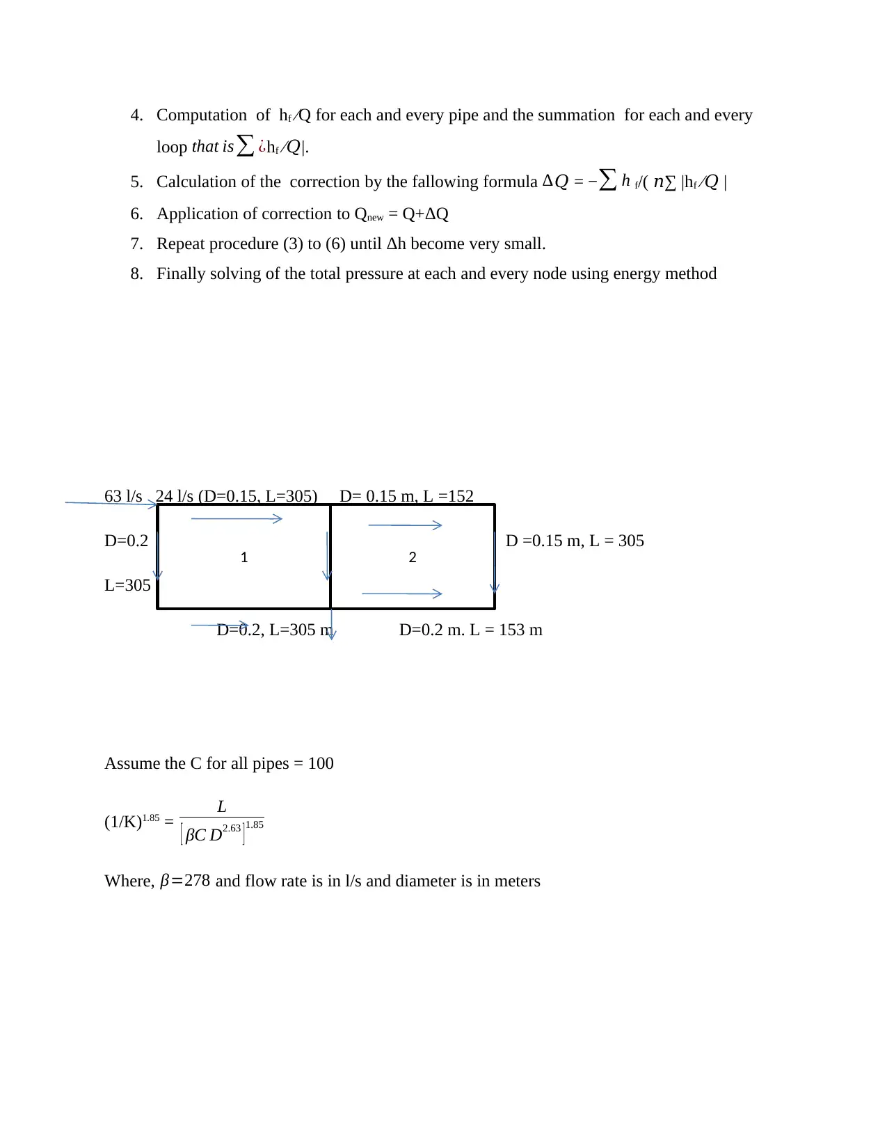
1st iteration
Loop Pipe Diameter
(m)
Length
(m)
(1/K)1.85 Q
(L/s)
H
(m)
H/Q
(m/L/s)
Correction
L/s
New Q
1 1 0.15 305 0.019 +24 +6.7 0.28 -0.24 +23.8
2 0.15 305 0.019 +11.4 +1.7 0.15 -2.4 +
0.57
+11.7
3 0.2 610 0.0092 -39 -8.1 0.21 -0.24 -39.2
Total +0.28 0.64
2 2 0.15 305 0.019 -11.4 -1.7 0.15 -0.57 +
0.24
-11.7
4 0.15 458 0.028 +12.6 +3.04 0.24 -0.57 +12.03
5 0.2 152 0.0023 -25.2 -0.9 0.04 -0.57 -25.8
Total +0.45 0.43
Qiteration 2loop 1=
−∑ H
n∑ H
Q
= −0.28
1.85∗0.64 = -0.24
Qiteration 1loop 2=
−∑ H
n∑ H
Q
= −0.45
1.85∗0.43 = -0.57

2st iteration
Loop Pipe Diameter
(m)
Length
(m)
(1/K)1.85 Q
(L/s)
H
(m)
H/Q
(m/L/s)
Correction
L/s
New
Q
1 1 0.15 305 0.019 +23.8 +6.6 0.28 -0.15 +23.6
2 0.15 305 0.019 +11.7 +1.8 0.15 -0.15 +
0.09
+11.7
3 0.2 610 0.0092 -39.2 -8.2 0.21 -0.15 -39.4
Total +0.18 0.64
2 2 0.15 305 0.019 -11.7 -1.8 0.15 -0.09 +
0.15
-11.7
4 0.15 458 0.028 +12.0 +2.8 0.23 -0.09 +11.9
5 0.2 152 0.0023 -25.8 -0.9 0.04 -0.09 -25.9
Total +0.07 0.42
Qiteration 2loop 1=
−∑ H
n∑ H
Q
= −0.18
1.85∗0.64 = -0.15
Qiteration 2loop 2=
−∑ H
n∑ H
Q
= −0.07
1.85∗0.42 = -0.09

PART B
DESIGN A SANITARY SEWER SYSTEM
Population in the initial years of the design period are low compared to the design population at
the end of design period
Peak flow rate in the initial years is low compared to the designed peak flow rate
Sizing should be such that it will attain the self-cleansing velocity at the average flow rate or at
least at the maximum flow rate at the beginning of the design period.
For Partially-full flow v is not influenced by the diameter of the pipe, rather is much influenced
by the slope of the channel
Average sewage flow Q = 0.8 * consumption
Qdesign = 2*peak factor * Q + infiltration (10%) + storm water (100% of peak flow)
Design equation using Manning`s formula (Vongvisessomjai, Tingsanchali and Babel, 2010) for
sewage flowing under gravity
V = 1
n∗¿ R2/3 * S1/2
Where,
V = velocity of flow in m/sec
R = hydraulic mean depth

S = slope of the sewer
n = coefficient of roughness for pipes (n = 0.013 for RCC pipes)
Cleansing velocity => for partially combined sewer = 0.7 m/sec
Maximum velocity used should not be greater than 2.4 m/sec, to avoid abrasion
Minimum sewer size to be used 225 mm to avoid chocking of sewer with bigger size objects
through the man hole
Minimum cover to be used = 1 m to avoid damage by live loads on sewer
Design procedure
1. Determination of present population of projected area
2. Drawing of the system layout while considering the streets and road layout.
3. Identification of the sewer line and numbering of the manhole.
4. Allocate plots to each sewer line
5. Measurement of the sewer line length as per scale of the map provided
6. Adopt the per capita sewage flow as 70% of water consumption and calculate the average
sewage flow and infiltration for all the sewer line., at this point take infiltration as 10% of
the average sewage flow
7. Calculation of peak sewage flow and design flow for the sewer lines (Hvitved-Jacobsen,
Vollertsen, and Nielsen, 2010)
8. By the usage of back calculation determine the appropriate diagram and sewer in
assumption that the sewer is fully flowing
9. In the end find the invert levels for all the sewer
10. Draw the profile for all sewer line

Data for design
Present year 2018 Design period 2038
Plots 7 10
Apartments 400 600
Flats 200 400
Assume the number of plots in the area = 280
Assume the number of apartment in the area = 3
Number of flats in the area = 3
Take the design period to be = 20 years
Present population = 7 * 28 + 400 * 3 + 200 * = 3767
Annual population growth rate for Australia = 1.98%
Population density in 2038 Pd = pp(1 + 1.98%) – 20 = 3822
Pd = 10*281 + 600 * 3 + 400 * 3 = 5810
Per capita water consumption = 300 lpc + 103 plc = 403 plc
Average sewer flow = pd * pcwc * 0.8/1000
= 5810 * 403 * 0.8/1000 = 1873 m3/day

= 0.0217 m3/s
Peak factor = 4
A = π∗¿(D/4)2
V = 1/N * R2/3 * S1/2
R = A/P = D/4
Q = A*V
Q=
π D2
4 ∗1
n ( D
4 )2
3∗S
1
2
Q = 0.0217 M3/S
S =0.001
N = 0.015
0.0217=
π D2
4 ∗1
0.015 ( D
4 ) 2
3∗0.001
1
2
D8/5 = 0.033022
D = 0.004267 M
D = 0.4 (TAKE)
V = Q/A
V = 0.0217/A
V = 1517 M/S which is greater than 0.6 m/s
Determination of manhole distance and pipe slope

Line A
Length = 100 m
Upper elevation = 70 m
Lower elevation = 68 m
S = ∆∈elevation
Length =70−68
100 = 0.02
Flow = 0.01217 m3/s
Diameter of the sewer line = 0.004267 m
Inverted at upper end = elevation – cover – diameter
Take cover = 3m
= 70 – 3 – 0.004267 = 66.996 m
Inverted at lower end = inverted at upper end – slope * length
= 66.996 – 0.02*100 = 64.996 m which is ok
Line B
Length = 100 m
S = ∆∈elevation
Length =68−64
100 = 0.04
Flow = 0.01217 m3/s
Diameter of the sewer line = 0.004267 m
Inverted at upper end = invert previously lower = 64.996 m
Inverted at lower end = inverted at upper end – slope * length
= 64.996 – 0.04*100 = 60.996 m which is ok

Line C
Length = 100 m
S = ∆∈elevation
Length =64−62
100 = 0.02
Flow = 0.01217 m3/s
Diameter of the sewer line = 0.004267 m
Inverted at upper end = elevation – cover – diameter
Take cover = 3m
= 60.996 – 3 – 0.004267 = 57.992 m
Inverted at lower end = inverted at upper end – slope * length
= 57.992 – 0.02*100 = 55.992 m which is ok
Line D
Length = 100 m
S = ∆∈elevation
Length =55.992−54
100 = 0.01992
Flow = 0.01217 m3/s
Diameter of the sewer line = 0.004267 m
Inverted at upper end = invert previously lower = 55.992 m
Inverted at lower end = inverted at upper end – slope * length
= 55.992 – 0.01992*100 = 54 m which is ok
Upper
manhole
Lower man
hole
Slope Upper invert
elevation
Lower invert
elevation
Length

Manhole A Manhole B 0.02 66.996 64.996 100
Manhole B Manhole C 0.04 64.996 60.996 100
Manhole C Manhole D 0.02 57.992 55.992 100
Manhole D Manhole E 0.01992 55.992 54 100
SANITARY SEWER LINE PROFILE
66.996
64.996
57.992
55.92

References
Baños, R., Gil, C., Reca, J. and Montoya, F.G., 2010. A memetic algorithm applied to the design
of water distribution networks. Applied Soft Computing, 10(1), pp.261-266
Cunha, M.D.C. and Sousa, J.J.D.O., 2010. Robust design of water distribution networks for a
proactive risk management. Journal of Water Resources Planning and Management, 136(2),
pp.227-236.
Giustolisi, O., 2010. Considering actual pipe connections in water distribution network
analysis. Journal of Hydraulic Engineering, 136(11), pp.889-900.
Huang, D., Vairavamoorthy, K. and Tsegaye, S., 2010. Flexible design of urban water
distribution networks. In World Environmental and Water Resources Congress 2010: Challenges
of Change (pp. 4225-4236).
Hvitved-Jacobsen, T., Vollertsen, J. and Nielsen, A.H., 2010. Urban and highway stormwater
pollution: Concepts and engineering. CRC press..
Joseph, D.D. and Yang, B.H., 2010. Friction factor correlations for laminar, transition and
turbulent flow in smooth pipes. Physica D: Nonlinear Phenomena, 239(14), pp.1318-1328.
Kumar, S.M., Narasimhan, S. and Bhallamudi, S.M., 2010. Parameter estimation in water
distribution networks. Water resources management, 24(6), pp.1251-1272.
Lisnianski, A., Frenkel, I. and Ding, Y., 2010. Multi-state system reliability analysis and
optimization for engineers and industrial managers. Springer Science & Business Media.
Spiliotis, M. and Tsakiris, G., 2010. Water distribution system analysis: Newton-Raphson
method revisited. Journal of Hydraulic Engineering, 137(8), pp.852-855.
Vongvisessomjai, N., Tingsanchali, T. and Babel, M.S., 2010. Non-deposition design criteria
for sewers with part-full flow. Urban Water Journal, 7(1), pp.61-77.