ENG3104: Engineering Simulations and Computations Assignment 2 - 2019

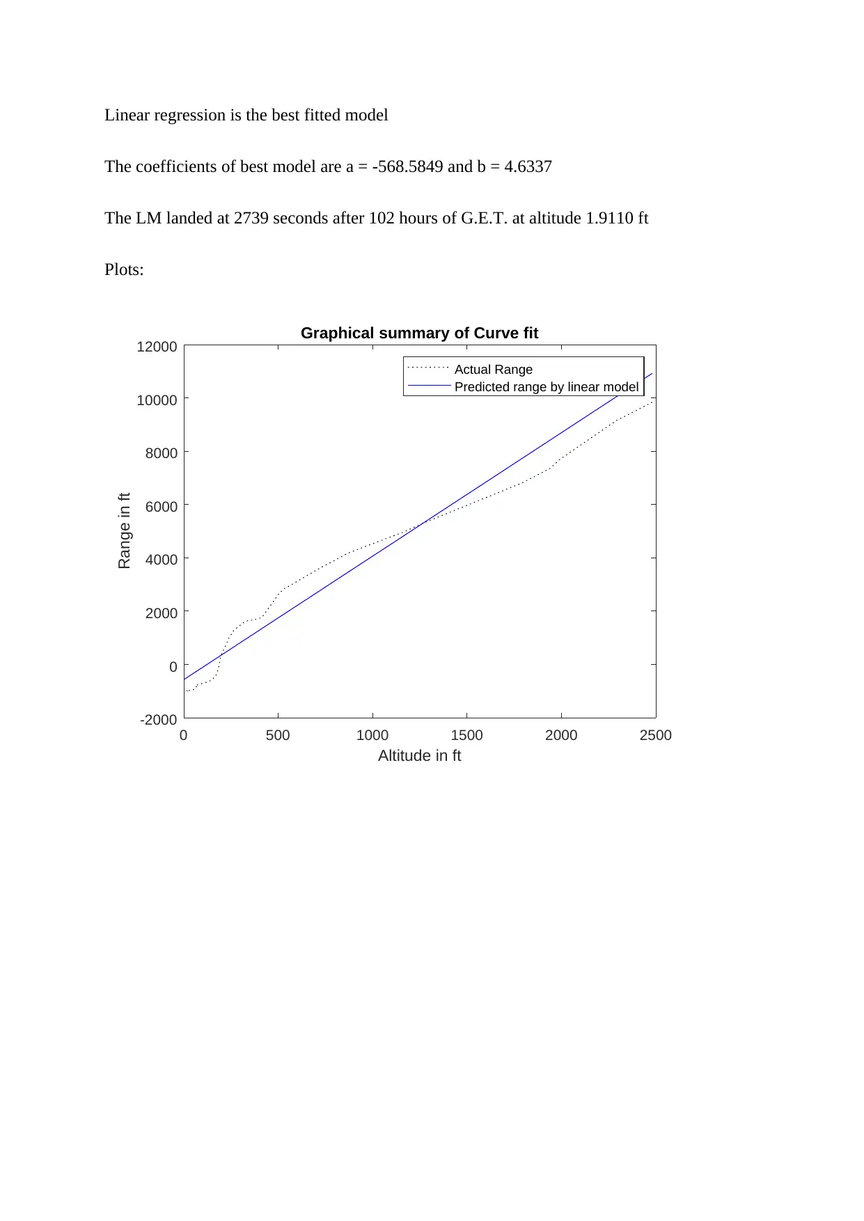
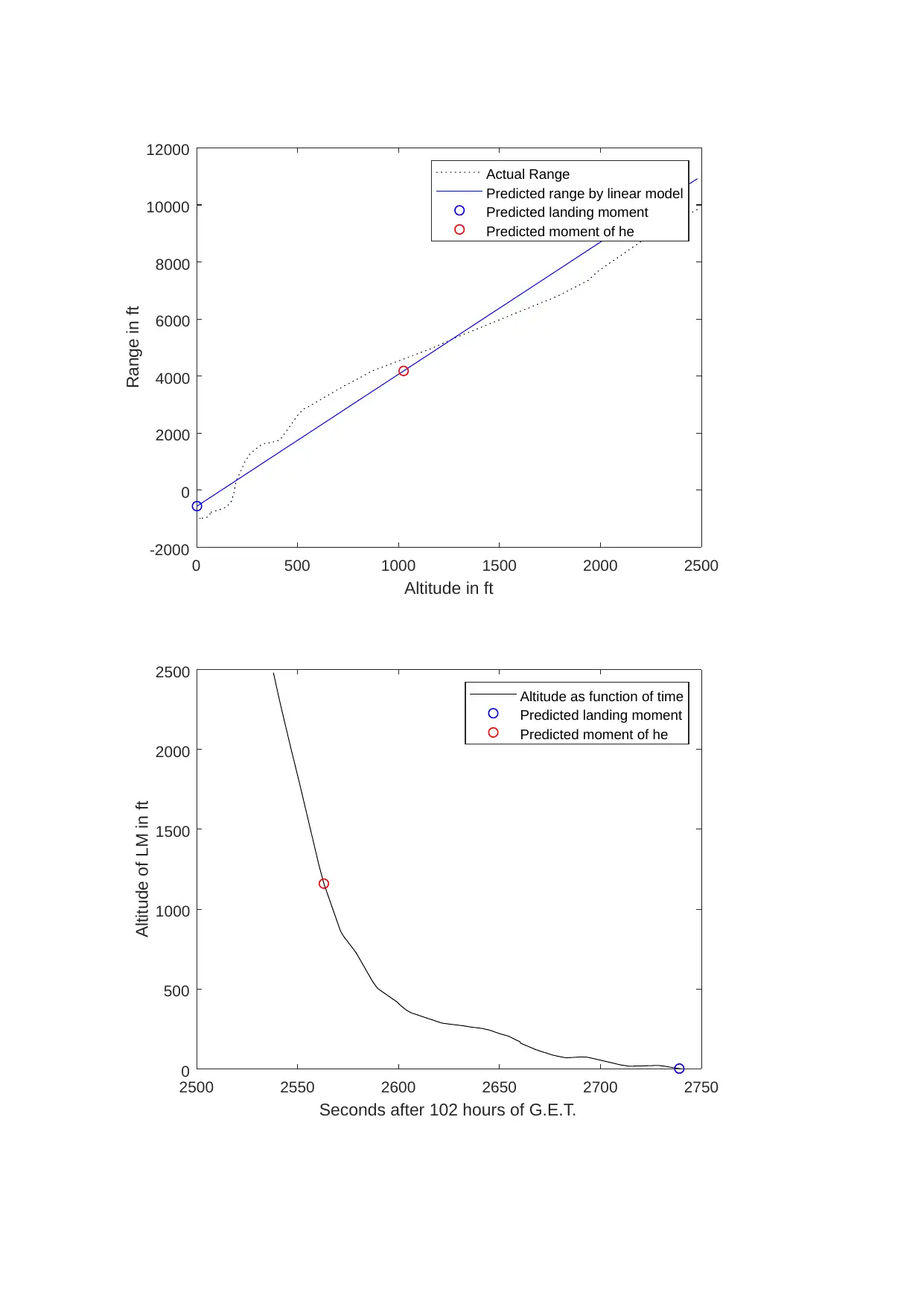
This document presents a comprehensive solution to Assignment 2 for the ENG3104 course on Engineering Simulations and Computations. The assignment focuses on analyzing the Apollo 11 Lunar Module (LM) during its landing. Question 1 involves calculating forces and moments using given acceleration and inertial properties, solved using both hand calculations and MATLAB. Question 2 explores curve fitting techniques to model the relationship between altitude and range using linear regression, logarithmic, and power series models, with MATLAB code for verification and analysis. Question 3 focuses on interpolation, specifically using linear interpolation and shape-preserving piecewise cubic interpolation to determine range and time at a specific altitude, supported by MATLAB code and comparison of results. The solution provides detailed calculations, MATLAB code, and graphical representations to illustrate the concepts and results.

Running head: ASSIGNMENT 2
ASSIGNMENT 2
Name of the Student
Name of the University
Author Note

Question 1:
Given, the acceleration of the lunar module is 0.5 m/s^2.
The properties of LM in Imperial units is given in the following table.
The mass of m of LM = 75665.2 lb = 75665.2*0.45359 = 34321.157 kgs.
Hence, F = 34321.157*0.5 = 17160.5785 N.
F1+F2=ma (2)
F2∗r2 – F1∗r1=I xx∗αx (3)
Given I xx = 19215 slug.ft^2 = 19215*1.3558 kg-m^2 = 26052.04 kg-m^2.
Now, linear acceleration in the positive y-direction is 0.5 m/s^2 or a = 0.5 m/s^2.
Now, the angular acceleration in x-direction is 0.25°/s^2 or αx = 0.25°/s^2 = 0.004 rad/s^2
F1+F2=34321.157∗0.5 (A)
Now, from figure 4, the distance of applied forces F1 and F2 from x axis is equal to 4.6’’.
Hence, r1 = r2 = 4.6’’ = 0.116 m.
Hence, substituting in equation (3)
F2∗0.116 – F1∗0.116=26052.04∗0.004
 F2 – F1 = 898.346 (B)
Now, solving (A) and (B) gives

F1 = 8131.1 N.
F2 = 9029.5 N.
Now, (2) and (3) in matrix form is given by,
[ 1 1
−r 1 r 2 ][ F 1
F 2 ] =
[ ma
I xx∗αx ]
Putting values,
[ 1 1
−0.116 0.116 ][ F 1
F 2 ] = [ 34321.157∗0.5
26052.04∗0.004 ]
Hence, [ F 1
F 2 ] = [ 1 1
−0.116 0.116 ]−1
[ 34321.157∗0.5
26052.04∗0.004 ]
[ F 1
F 2 ] = [ 8131.1
9029.5 ]
The above results are verified by MATLAB as given below.
MATLAB code:
a = 0.5; % acceleration in m/s^2
m = 75665.2*0.45359; % mass of LM
format shortG
F = m*a
r1 = 0.116; r2 = r1; % the distance of applied forces F1 and F2 from x axis
Ixx = 19215*1.3558; % moment of inertia about x axis in kg-m^2
alphax = (0.25*pi)/180; % angular acceletation in rad/s^2

A = [1,1;-0.116,0.116]; B = [m*a;Ixx*alphax];
F = A^(-1)*B;
F1 = F(1)
F2 = F(2)
Output:
q1r4
F =
17160
F1 =
8090.3
F2 =
9070.2
Question 2:
The first two values of altitude when alarm 1201 was active are 2480 ft and 2290 ft
respectively. Also, at the same instants the range in ft are 9840 ft and 9150 ft respectively.
Now, by linear regression of curve fitting the range as a function of altitude will be.
Range = a + b*alt
a = ((∑ y ¿∗(∑ x2 )−(∑ x )(∑ xy )¿ /¿ = 833.68
b = (n( ∑ xy ¿−(∑ x )(∑ y )¿ /¿ = 3.6316

Now, by fitting logarithmic function to the data
Range = a + b*ln(alt)
The estimates of a and b will be
Range = -57821 + 8656.7*ln(alt)
Now, power series is fitted with the data.
Range=a∗ ( alt ) b
The estimates of a and b will be
Range=7.886∗( alt )0.9121
MATLAB code for verification:
range = [9840,9150]; alt = [2480,2290];
linmod = fitlm(alt,range) % linear regression model Range = a + b*alt form
lnalt = log(alt);
logmod = fitlm(lnalt,range) % logarithmic model
powmod = fit(alt',range','power1') % power series model
Output:
q2r2
linmod =
Linear regression model:
y ~ 1 + x1

Estimated Coefficients:
Estimate SE tStat pValue
________ __ _____ ______
(Intercept) 833.68 0 Inf NaN
x1 3.6316 0 Inf NaN
Number of observations: 2, Error degrees of freedom: 0
R-squared: 1, Adjusted R-Squared NaN
F-statistic vs. constant model: NaN, p-value = NaN
logmod =
Linear regression model:
y ~ 1 + x1
Estimated Coefficients:
Estimate SE tStat pValue
________ __ _____ ______
(Intercept) -57821 0 -Inf NaN
x1 8656.7 0 Inf NaN
Number of observations: 2, Error degrees of freedom: 0
R-squared: 1, Adjusted R-Squared NaN
F-statistic vs. constant model: NaN, p-value = NaN
powmod =

General model Power1:
powmod(x) = a*x^b
Coefficients:
a = 7.886
b = 0.9121
MATLAB code:
[num,txt,raw] = xlsread('Apollo11landing.csv','A8:E153');
time = cellstr(string(raw(29:end,1)));infmt = 'mm:ss.SSS'; dur =
seconds(duration(time,'InputFormat',infmt));
Altitude = num(29:end,1)+0.001; % offsetting range by negligible 0.001 fts for normalization
Range = num(29:end,2);
%% linear model fit
tbl = table(Altitude,Range,'VariableNames',{'Altitude','Range'});
linmod = fitlm(tbl,'Range~1+Altitude');
%% logarithimic model fit
lnalt = log(Altitude);
tbl = table(lnalt,Range,'VariableNames',{'Log_Altitude','Range'});
logmod = fitlm(tbl,'Range~1+Log_Altitude');

%% Power model fit
[powmod,gof] = fit(Altitude,Range,'power1'); % power series model
%% Displaying numerical test results of three model
fprintf('R^2 of linear model = %.4f.\n R^2 of logarithimic model = %.4f.\n R^2 of power
series model = %.4f.\n',linmod.Rsquared.Ordinary,logmod.Rsquared.Ordinary,...
gof.rsquare)
fprintf('RMSE of linear model = %.4f.\n RMSE of logarithimic model = %.4f.\n RMSE of
power series model = %.4f.\n',linmod.RMSE,logmod.RMSE,...
gof.rmse)
fprintf('Linear regression is the best fitted model\n'); coeff = linmod.Coefficients.Estimate;
fprintf('The coefficients of best model are a = %.4f and b = %.4f \n',coeff(1),coeff(2))
%% Plotting best fit model with data
Rangepred = coeff(1) + Altitude.*coeff(2);
figure(1)
plot(Altitude,Range,'k:',Altitude,Rangepred,'b-')
legend('Actual Range','Predicted range by linear model')

xlabel('Altitude in ft')
ylabel('Range in ft')
title('Graphical summary of Curve fit')
%% predicting he and landing time of LM by best curve
fprintf('The LM landed at %d seconds after 102 hours of G.E.T. at altitide %.4f\n',dur(end-
1),Altitude(end-1))
he = (10 + 0.24839)*100;
rangeathe = coeff(1) + he*coeff(2);
%% plot of calculated data
figure(2)
plot(Altitude,Range,'k:',Altitude,Rangepred,'b-',Altitude(end-1),Rangepred(end-
1),'bo',he,rangeathe,'ro')
legend('Actual Range','Predicted range by linear model','Predicted landing moment','Predicted
moment of he')
xlabel('Altitude in ft')
ylabel('Range in ft')

%% finding instant in which altitude is closest to he
diffalt = abs(Altitude - he);
for i=1:length(Altitude)
if diffalt(i) == min(diffalt)
index = i;
end
end
figure(3)
plot(dur,Altitude,'k-',dur(end-1),Altitude(end-1),'bo',dur(index),Altitude(index),'ro')
xlabel('Seconds after 102 hours of G.E.T.')
ylabel('Altitude of LM in ft')
legend('Altitude as function of time','Predicted landing moment','Predicted moment of he')
Output:
R^2 of linear model = 0.9183.
R^2 of logarithimic model = 0.4225.
R^2 of power series model = 0.8745.
RMSE of linear model = 601.0500.
RMSE of logarithimic model = 1597.8098.
RMSE of power series model = 744.7739.

Linear regression is the best fitted model
The coefficients of best model are a = -568.5849 and b = 4.6337
The LM landed at 2739 seconds after 102 hours of G.E.T. at altitude 1.9110 ft
Plots:
0 500 1000 1500 2000 2500
Altitude in ft
-2000
0
2000
4000
6000
8000
10000
12000
Range in ft
Graphical summary of Curve fit
Actual Range
Predicted range by linear model

0 500 1000 1500 2000 2500
Altitude in ft
-2000
0
2000
4000
6000
8000
10000
12000
Range in ft
Actual Range
Predicted range by linear model
Predicted landing moment
Predicted moment of he
2500 2550 2600 2650 2700 2750
Seconds after 102 hours of G.E.T.
0
500
1000
1500
2000
2500
Altitude of LM in ft
Altitude as function of time
Predicted landing moment
Predicted moment of he

Question 3:
Q3 = 7:693 > 5 (hence, shape-preserving piecewise cubic interpolation method will be used)
The formula for linear interpolation is given by,
y2 = ((x2-x1)(y3-y1))/(x3-x1) + y1
Now, for the case of interpolation x2 = 2500 ft and the two adjacent points in the altitude list
are 2930 ft and 2480 ft at which ranges are 11400 ft and 9840 ft.
Hence, range at 2500 ft = ((2500-2930)(9840-11400))/(2480-2930) + 11400 = 9909.3 ft.
Now, time just before and after of 2500 ft altitude are 2538 secs and 2541.4 secs with altitude
2930 ft and 2480 ft respectively.
y2 = ((2500-2930)*(2541.4-2538))/(2480-2930) + 2538 = 2541.2 secs.
MATLAB code for verification:
x1=2930; x2 = 2500; x3 = 2480;
y1 = 11400; y3 = 9840;
y2 = ((x2-x1)*(y3-y1))/(x3-x1) + y1;
fprintf('The range at 2500 ft is %.1f ft\n',y2)
y1 = 2538; y3 = 2541.4;
y2 = ((x2-x1)*(y3-y1))/(x3-x1) + y1;
fprintf('The time after 102 hours of G.E.T at 2500 ft is %.1f secs\n',y2)

Output:
The range at 2500 ft is 9909.3 ft
The time after 102 hours of G.E.T at 2500 ft is 2541.2 secs
MATLAB code:
[num,txt,raw] = xlsread('Apollo11landing.csv','A8:E153');
time = cellstr(string(raw(24:end,1)));infmt = 'mm:ss.SSS'; dur =
seconds(duration(time,'InputFormat',infmt));
Altitude = num(24:end,1); Range = num(24:end,2);
%% Filtering repeated values
[alfilt, ia, ic] = unique(Altitude,'stable');
for i=1:length(ia)
rangefilt(i) = Range(ia(i));
durfilt(i) = dur(ia(i));
end
%% spline interpolation and shape-preserving piecewise cubic interpolation
rangefilt = rangefilt';durfilt = durfilt';
h = 2500;
rangesp = spline(alfilt,rangefilt,h);

rangepchip = pchip(alfilt,rangefilt,h);
plot(alfilt,rangefilt,'b-',h,rangesp,'k*',h,rangepchip,'ro','MarkerSize',10)
xlabel('Altitude in ft')
ylabel('Range in ft')
legend('Original data','Range predicted at 2500 ft by spline','Range predicted at 2500 ft by
shape-preserving piecewise cubic interpolation')
fprintf('The range predicted at 2500 ft Altitude by spline interpolation is %.4f ft and shape-
preserving piecewise cubic interpolation is %.4f ft \n',rangesp,rangepchip)
he = (10 + 0.24839)*100;
rangesp = spline(alfilt,rangefilt,he);
rangepchip = pchip(alfilt,rangefilt,he);
fprintf('The range predicted at he =%.4f ft by spline interpolation is %.4f ft and shape-
preserving piecewise cubic interpolation is %.4f ft\n',he,rangesp,rangepchip)
Output:
The range predicted at 2500 ft Altitude by spline interpolation is 9910.9494 ft and shape-
preserving piecewise cubic interpolation is 9911.0609 ft
The range predicted at he =1024.8390 ft by spline interpolation is 4632.7217 ft and shape-
preserving piecewise cubic interpolation is 4611.0428 ft
Plot:

0 1000 2000 3000 4000 5000 6000 7000
Altitude in ft
-0.5
0
0.5
1
1.5
2
2.5
3
Range in ft
104
Original data
Range predicted at 2500 ft by spline
Range predicted at 2500 ft by shape-preserving piecewise cubic interpolation