Engineering and Computing MATLAB Assignment, Spring 2019
VerifiedAdded on 2023/04/21
|19
|2788
|110
Homework Assignment
AI Summary
This document presents a comprehensive MATLAB assignment solution for an Engineering and Computing course, likely from Spring 2019. The assignment covers a range of topics, including plotting mathematical functions (sinh(x)), analyzing electrical circuits, solving quadratic equations using matrix inversion, numerical solutions of differential equations using Euler's method, and simulating physical systems. The solution provides MATLAB code, plots, and detailed explanations for each problem, demonstrating the application of MATLAB in various engineering contexts. Specific problems include circuit analysis, curve fitting, solving differential equations using numerical methods, and calculating mass flow rate through a converging nozzle. The code and plots are presented with clear labeling and formatting for easy understanding.
Running head: ENGINEERING AND COMPUTING
ENGINEERING AND COMPUTING
Name of the Student
Name of the University
Author Note
ENGINEERING AND COMPUTING
Name of the Student
Name of the University
Author Note
Paraphrase This Document
Need a fresh take? Get an instant paraphrase of this document with our AI Paraphraser
1ENGINEERING AND COMPUTING
Question 1:
MATLAB script:
clc
clear
disp('Question No 1: Your Name,Spring,2019')
x=-2*pi:0.1:2*pi;
y1 = sinh(x);
y2 = (exp(x) - exp(-x))/2;
plot(x,y1,'r-',x,y2,'b*')
legend('y1','y2')
title('Plot of sinh(x) and (e^{x} - e^{-x})/2')
xlabel('x in range -2\pi to 2\pi')
ylabel('y1 and y2')
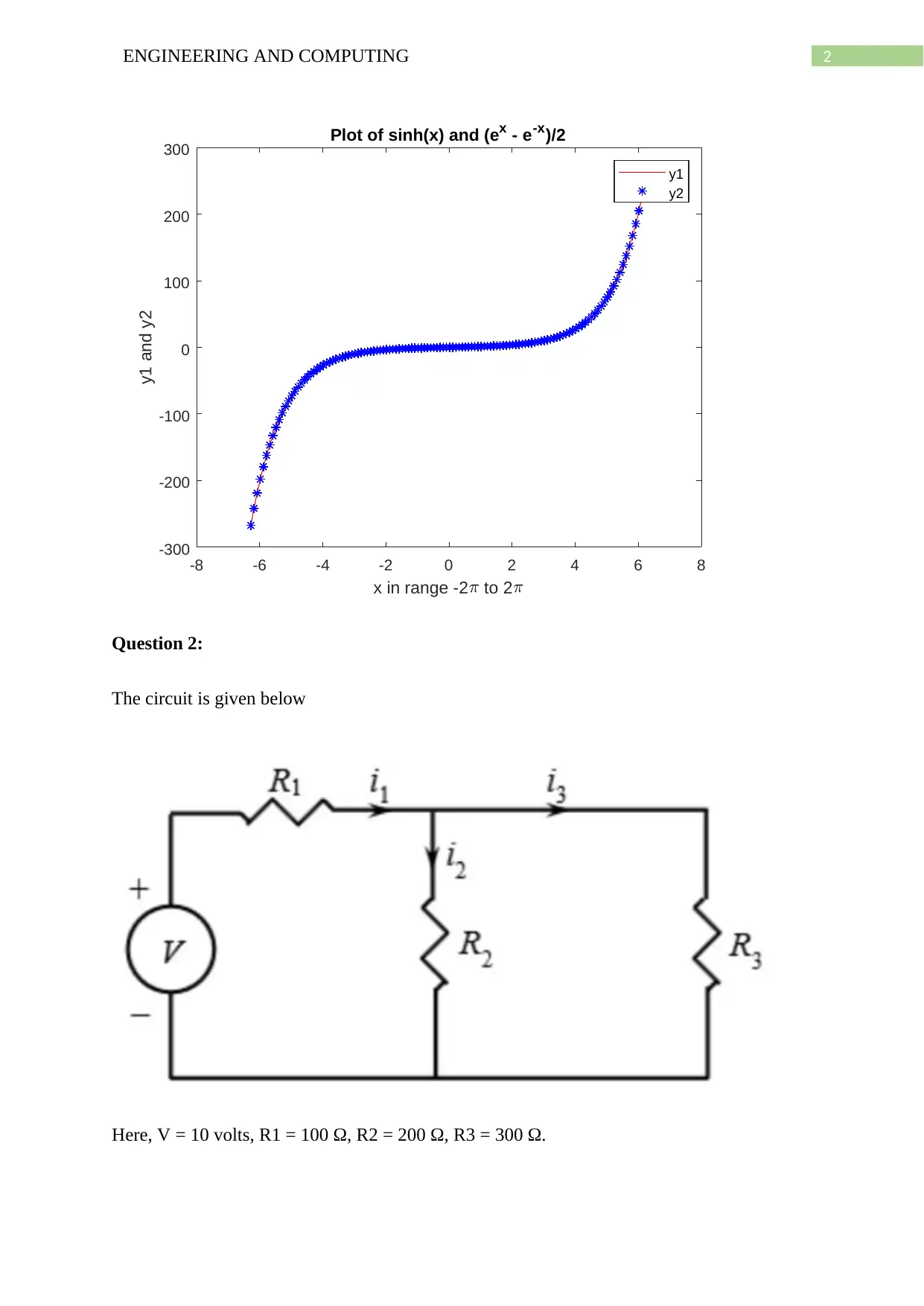
Plot:
Question 1:
MATLAB script:
clc
clear
disp('Question No 1: Your Name,Spring,2019')
x=-2*pi:0.1:2*pi;
y1 = sinh(x);
y2 = (exp(x) - exp(-x))/2;
plot(x,y1,'r-',x,y2,'b*')
legend('y1','y2')
title('Plot of sinh(x) and (e^{x} - e^{-x})/2')
xlabel('x in range -2\pi to 2\pi')
ylabel('y1 and y2')
Plot:
2ENGINEERING AND COMPUTING
-8 -6 -4 -2 0 2 4 6 8
x in range -2 to 2
-300
-200
-100
0
100
200
300
y1 and y2
Plot of sinh(x) and (ex - e-x)/2
y1
y2
Question 2:
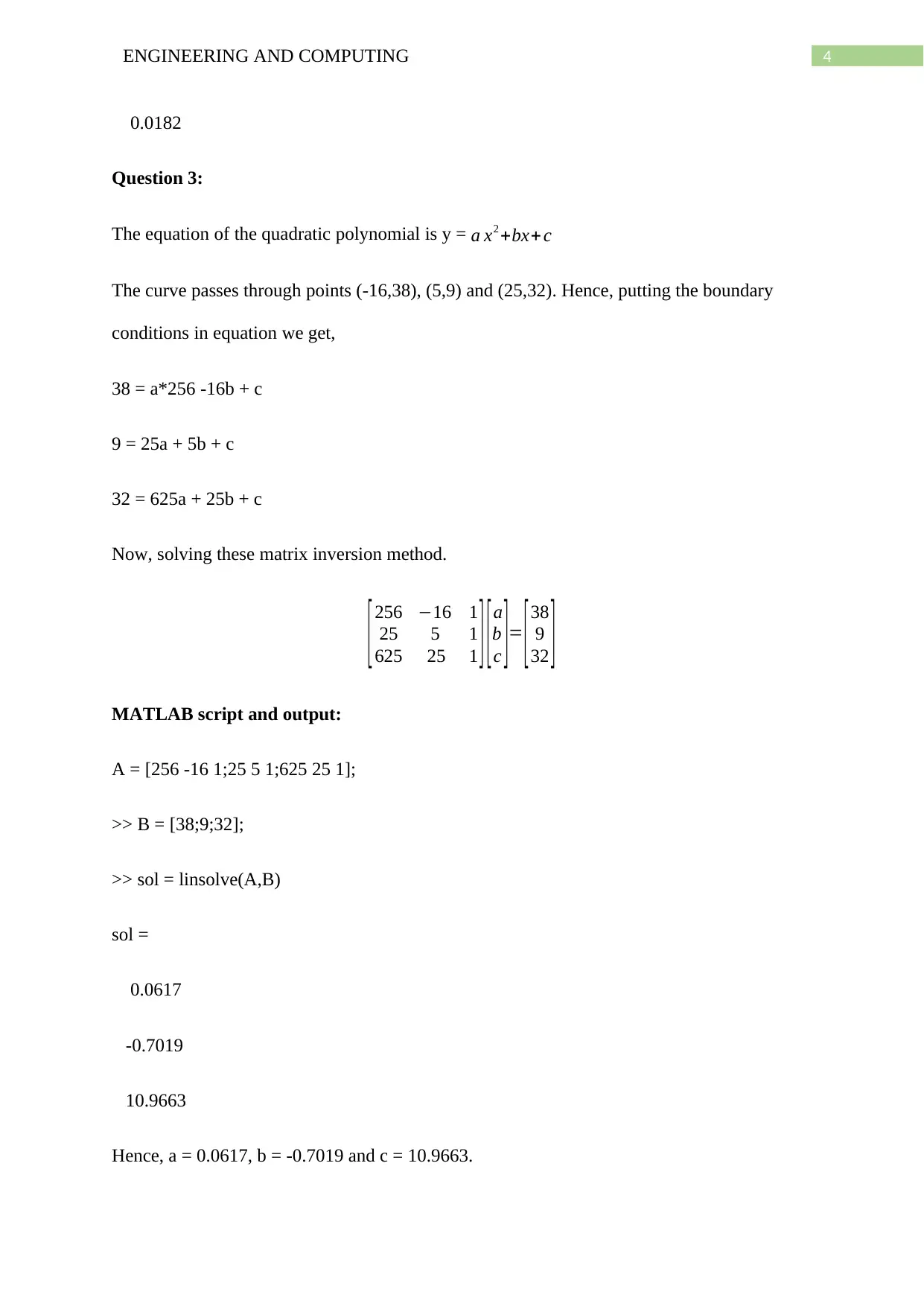
The circuit is given below
Here, V = 10 volts, R1 = 100 Ω, R2 = 200 Ω, R3 = 300 Ω.
-8 -6 -4 -2 0 2 4 6 8
x in range -2 to 2
-300
-200
-100
0
100
200
300
y1 and y2
Plot of sinh(x) and (ex - e-x)/2
y1
y2
Question 2:
The circuit is given below
Here, V = 10 volts, R1 = 100 Ω, R2 = 200 Ω, R3 = 300 Ω.
⊘ This is a preview!⊘
Do you want full access?
Subscribe today to unlock all pages.

Trusted by 1+ million students worldwide
3ENGINEERING AND COMPUTING
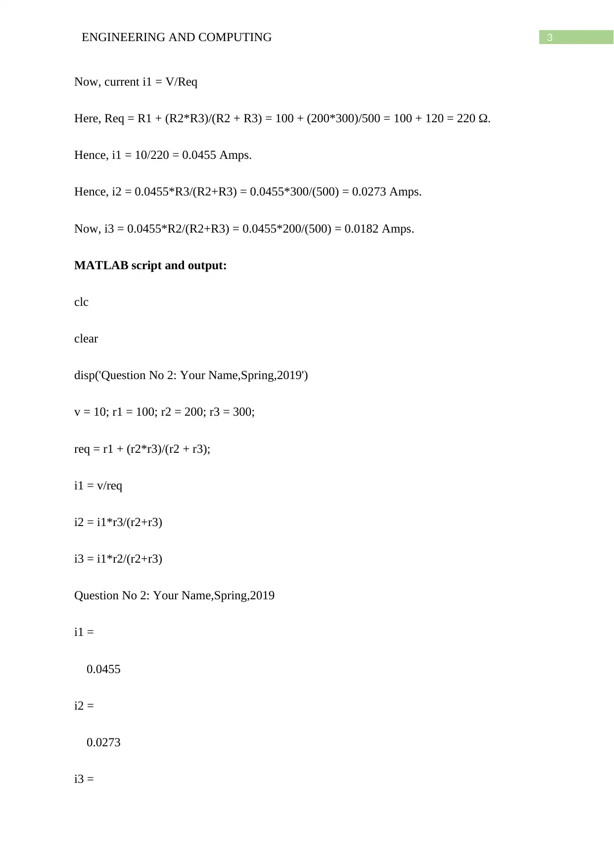
Now, current i1 = V/Req
Here, Req = R1 + (R2*R3)/(R2 + R3) = 100 + (200*300)/500 = 100 + 120 = 220 Ω.
Hence, i1 = 10/220 = 0.0455 Amps.
Hence, i2 = 0.0455*R3/(R2+R3) = 0.0455*300/(500) = 0.0273 Amps.
Now, i3 = 0.0455*R2/(R2+R3) = 0.0455*200/(500) = 0.0182 Amps.
MATLAB script and output:
clc
clear
disp('Question No 2: Your Name,Spring,2019')
v = 10; r1 = 100; r2 = 200; r3 = 300;
req = r1 + (r2*r3)/(r2 + r3);
i1 = v/req
i2 = i1*r3/(r2+r3)
i3 = i1*r2/(r2+r3)
Question No 2: Your Name,Spring,2019
i1 =
0.0455
i2 =
0.0273
i3 =
Paraphrase This Document
Need a fresh take? Get an instant paraphrase of this document with our AI Paraphraser
4ENGINEERING AND COMPUTING
0.0182
Question 3:
The equation of the quadratic polynomial is y = a x2 +bx+ c
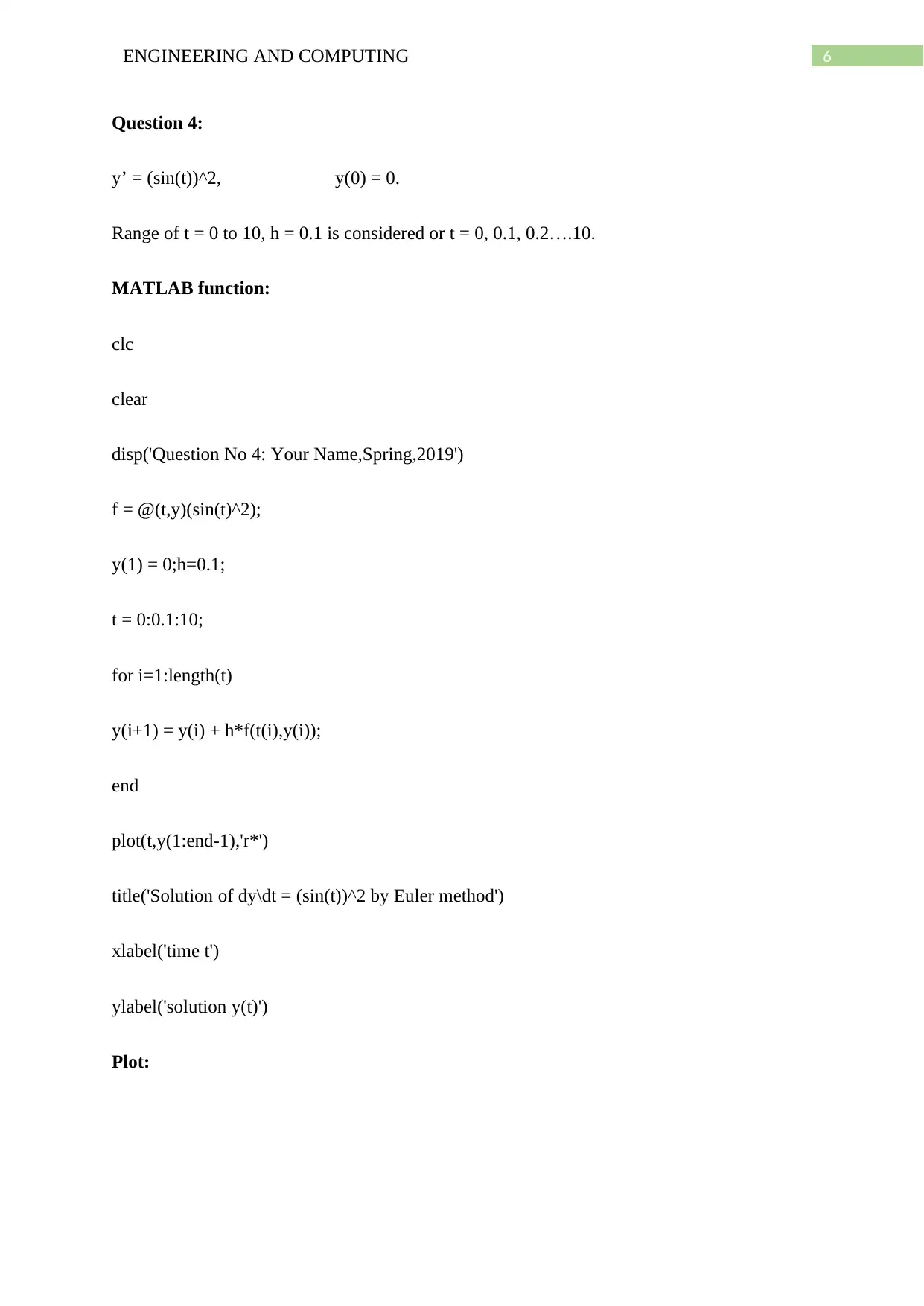
The curve passes through points (-16,38), (5,9) and (25,32). Hence, putting the boundary
conditions in equation we get,
38 = a*256 -16b + c
9 = 25a + 5b + c
32 = 625a + 25b + c
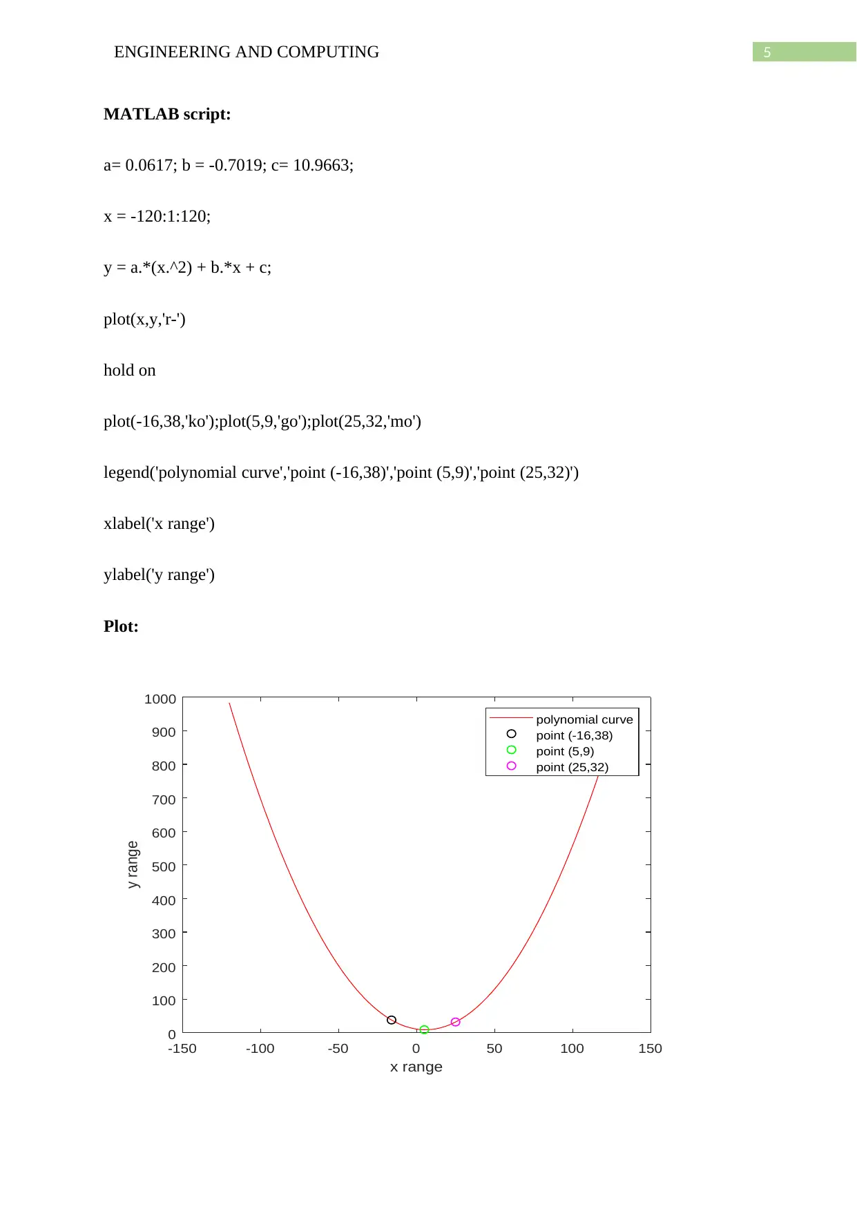
Now, solving these matrix inversion method.
[256 −16 1
25 5 1
625 25 1 ][a
b
c ]= [38
9
32 ]
MATLAB script and output:
A = [256 -16 1;25 5 1;625 25 1];
>> B = [38;9;32];
>> sol = linsolve(A,B)
sol =
0.0617
-0.7019
10.9663
Hence, a = 0.0617, b = -0.7019 and c = 10.9663.
5ENGINEERING AND COMPUTING
MATLAB script:
a= 0.0617; b = -0.7019; c= 10.9663;
x = -120:1:120;
y = a.*(x.^2) + b.*x + c;
plot(x,y,'r-')
hold on
plot(-16,38,'ko');plot(5,9,'go');plot(25,32,'mo')
legend('polynomial curve','point (-16,38)','point (5,9)','point (25,32)')
xlabel('x range')
ylabel('y range')
Plot:
-150 -100 -50 0 50 100 150
x range
0
100
200
300
400
500
600
700
800
900
1000
y range
polynomial curve
point (-16,38)
point (5,9)
point (25,32)
⊘ This is a preview!⊘
Do you want full access?
Subscribe today to unlock all pages.

Trusted by 1+ million students worldwide
6ENGINEERING AND COMPUTING
Question 4:
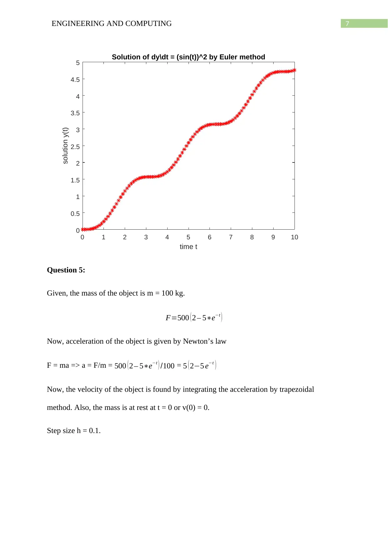
y’ = (sin(t))^2, y(0) = 0.
Range of t = 0 to 10, h = 0.1 is considered or t = 0, 0.1, 0.2….10.
MATLAB function:
clc
clear
disp('Question No 4: Your Name,Spring,2019')
f = @(t,y)(sin(t)^2);
y(1) = 0;h=0.1;
t = 0:0.1:10;
for i=1:length(t)
y(i+1) = y(i) + h*f(t(i),y(i));
end
plot(t,y(1:end-1),'r*')
title('Solution of dy\dt = (sin(t))^2 by Euler method')
xlabel('time t')
ylabel('solution y(t)')
Plot:
Paraphrase This Document
Need a fresh take? Get an instant paraphrase of this document with our AI Paraphraser
7ENGINEERING AND COMPUTING
0 1 2 3 4 5 6 7 8 9 10
time t
0
0.5
1
1.5
2
2.5
3
3.5
4
4.5
5
solution y(t)
Solution of dy\dt = (sin(t))^2 by Euler method
Question 5:
Given, the mass of the object is m = 100 kg.
F=500 ( 2 – 5∗e−t )
Now, acceleration of the object is given by Newton’s law
F = ma => a = F/m = 500 ( 2 – 5∗e−t ) /100 = 5 ( 2−5 e−t )
Now, the velocity of the object is found by integrating the acceleration by trapezoidal
method. Also, the mass is at rest at t = 0 or v(0) = 0.
Step size h = 0.1.
8ENGINEERING AND COMPUTING
MATLAB code:
clc
clear
disp('Question No 5: Your Name,Spring,2019')
h=0.1;
a = @(t) (5*(2-5*exp(t)));
t= 0:h:5;
for i =1:(length(t)-1)
v(i+1) = (h/2)*(a(t(i)) + a(t(i+1)));
acc(i) = a(t(i));
end
plot(t,v,'r*',t(1:(end-1)),acc,'b*')
legend('v(t)','a(t)')
title('Plot of velocity and accleration as a function of time')
xlabel('time t in 0 to 5 sec')
ylabel('v(t) and a(t)')
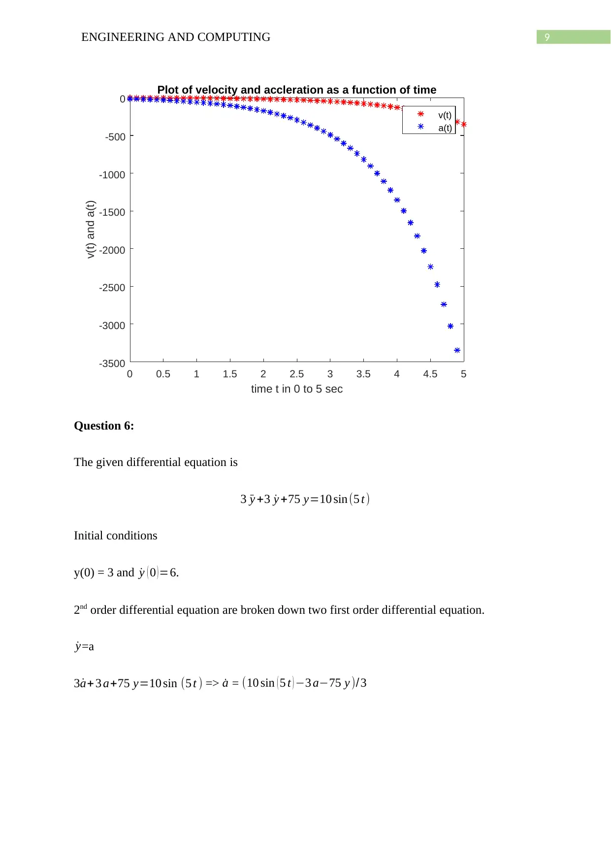
Plot of velocity and acceleration w.r.t time:
⊘ This is a preview!⊘
Do you want full access?
Subscribe today to unlock all pages.

Trusted by 1+ million students worldwide
9ENGINEERING AND COMPUTING
0 0.5 1 1.5 2 2.5 3 3.5 4 4.5 5
time t in 0 to 5 sec
-3500
-3000
-2500
-2000
-1500
-1000
-500
0
v(t) and a(t)
Plot of velocity and accleration as a function of time
v(t)
a(t)
Question 6:
The given differential equation is
3 ¨y +3 ˙y +75 y=10 sin(5 t )
Initial conditions
y(0) = 3 and ˙y ( 0 )=6.
2nd order differential equation are broken down two first order differential equation.
˙y=a
3 ˙a+3 a+75 y=10 sin (5 t ) => ˙a = (10 sin ( 5 t ) −3 a−75 y )/3
Paraphrase This Document
Need a fresh take? Get an instant paraphrase of this document with our AI Paraphraser
10ENGINEERING AND COMPUTING
MATLAB function:
clc
clear
disp('Question No 6: Your Name,Spring,2019')
h = 0.1;
dy = @(t,a) (a);
d2y = @(a,t,y) (10*sin(5*t) - 3*a - 75*y)/3;
a(1) = 6; y(1) = 3;
t = 0:0.1:10;
for i=1:length(t)
y(i+1) = y(i) + h*dy(t(i),a(i));
a(i+1) = a(i) + h*d2y(a(i),t(i),y(i));
end
plot(t,a(1:end-1),'r-',t,y(1:end-1),'b-')
legend('dy/dt','y')
xlabel('time t')
ylabel('dy/dt and y')
11ENGINEERING AND COMPUTING
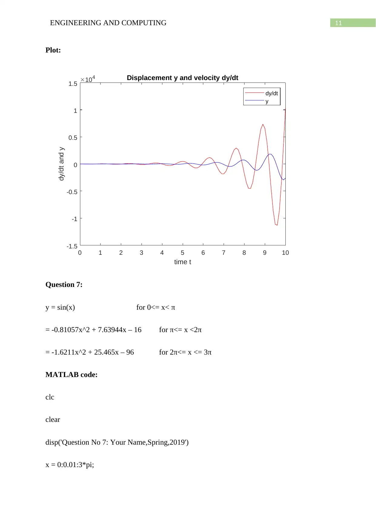
Plot:
0 1 2 3 4 5 6 7 8 9 10
time t
-1.5
-1
-0.5
0
0.5
1
1.5
dy/dt and y
104 Displacement y and velocity dy/dt
dy/dt
y
Question 7:
y = sin(x) for 0<= x< π
= -0.81057x^2 + 7.63944x – 16 for π<= x <2π
= -1.6211x^2 + 25.465x – 96 for 2π<= x <= 3π
MATLAB code:
clc
clear
disp('Question No 7: Your Name,Spring,2019')
x = 0:0.01:3*pi;
⊘ This is a preview!⊘
Do you want full access?
Subscribe today to unlock all pages.

Trusted by 1+ million students worldwide
1 out of 19
Your All-in-One AI-Powered Toolkit for Academic Success.
+13062052269
info@desklib.com
Available 24*7 on WhatsApp / Email
![[object Object]](/_next/static/media/star-bottom.7253800d.svg)
Unlock your academic potential
Copyright © 2020–2026 A2Z Services. All Rights Reserved. Developed and managed by ZUCOL.


