Civil Engineering Hydrology Report: Flow Rate and Baseflow Analysis
VerifiedAdded on 2023/01/19
|22
|5676
|28
Report
AI Summary
This report provides a detailed analysis of key concepts in engineering hydrology. It begins by discussing the impact of the water cycle on the environment, emphasizing its role in regulating plant, animal, and human life. The report then explores various methods for measuring flow rate in natural watercourses, including the eyeball method, depth to flow method, immersed current meter, surface velocity area method, artificial tracing method, and primary device method, comparing their accuracy and suitability for different scenarios. Finally, the report outlines the straight line method for separating base flow from a stream's hydrograph, a crucial step in understanding runoff dynamics. The report covers the impact of climate change on the water cycle, and the methods used for flow measurement are presented with their advantages and disadvantages. The report also includes a brief overview of how to estimate the value of the 1-in-50-year flow, and the components of a hydrograph.

Engineering Hydrology 1
ENGINEERING HYDROLOGY
Name
Course
Professor
University
City/state
Date
ENGINEERING HYDROLOGY
Name
Course
Professor
University
City/state
Date
Paraphrase This Document
Need a fresh take? Get an instant paraphrase of this document with our AI Paraphraser
Engineering Hydrology 2
Engineering Hydrology
Task 1
a) Impact of water cycle on the environment
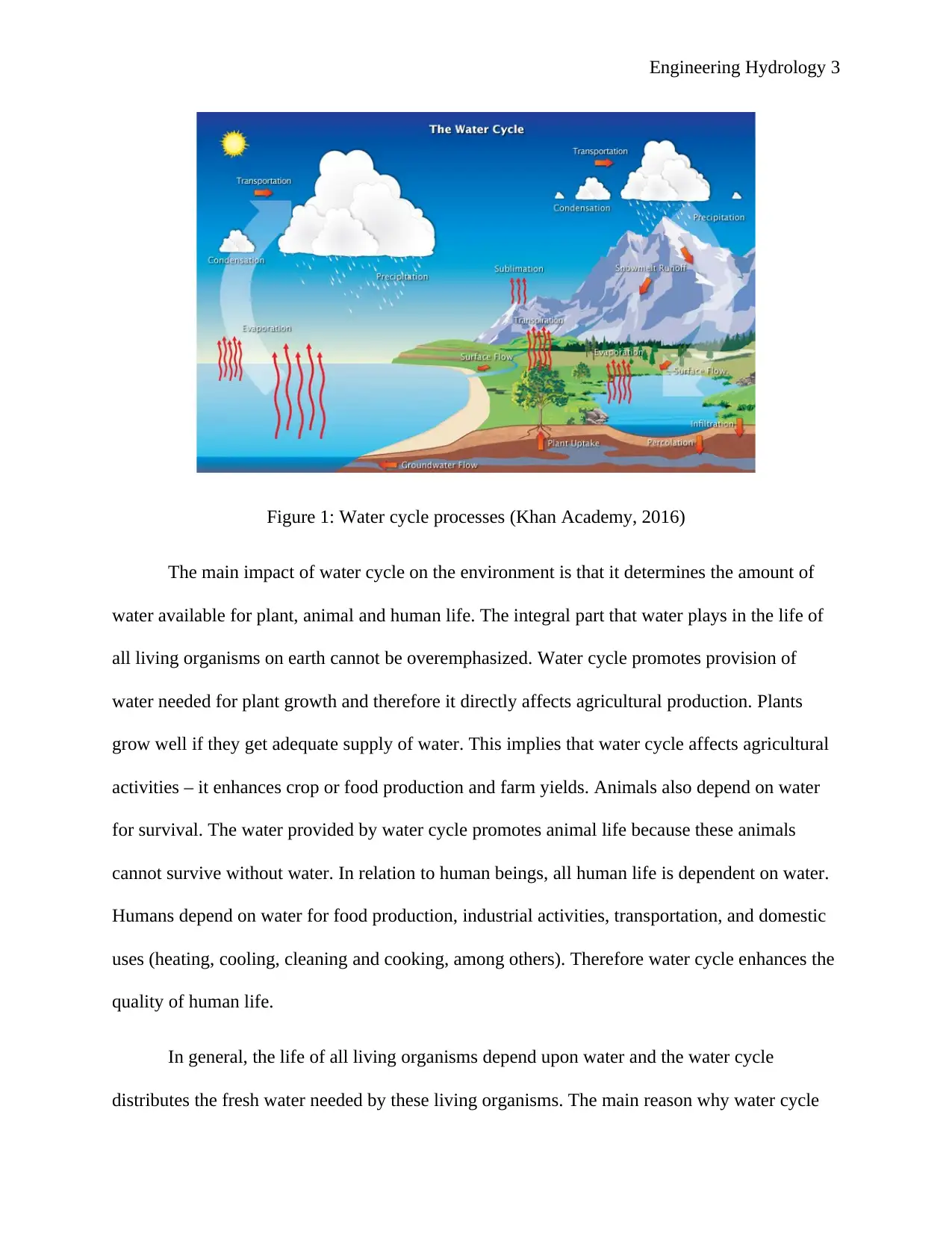
Most or all the water that the earth receives is as a result of water cycle. Water cycle is a
virtuous cycle that starts with evaporation of water from any watercourses such as oceans, rivers,
streams or seas and transpiration from soils and plants, after being heated by the sun. The
evaporated water rises up into the atmosphere as a gas (water vapour) and then starts cooling and
condensing after reaching a certain height to become clouds. The clouds continue accumulating
and when they become heavy enough, they fall back onto the earth as precipitation (Supriya,
(n.d.)). The precipitation, which is in form of rain, is a very essential component for human, plant
and animal life. After falling onto the surface of the earth, the water runs off back to
watercourses where it evaporates again and the process repeats itself making water to circulate
continuously in the earth-atmosphere system (IPCC, 2013). The water cycle processes are
presented in Figure 1 below. Therefore water cycle is a complex but very essential constituent of
the planetary system that plays a key role in regulating human, plant and animal life (Sohoulande
& Singh, 2015).
Engineering Hydrology
Task 1
a) Impact of water cycle on the environment
Most or all the water that the earth receives is as a result of water cycle. Water cycle is a
virtuous cycle that starts with evaporation of water from any watercourses such as oceans, rivers,
streams or seas and transpiration from soils and plants, after being heated by the sun. The
evaporated water rises up into the atmosphere as a gas (water vapour) and then starts cooling and
condensing after reaching a certain height to become clouds. The clouds continue accumulating
and when they become heavy enough, they fall back onto the earth as precipitation (Supriya,
(n.d.)). The precipitation, which is in form of rain, is a very essential component for human, plant
and animal life. After falling onto the surface of the earth, the water runs off back to
watercourses where it evaporates again and the process repeats itself making water to circulate
continuously in the earth-atmosphere system (IPCC, 2013). The water cycle processes are
presented in Figure 1 below. Therefore water cycle is a complex but very essential constituent of
the planetary system that plays a key role in regulating human, plant and animal life (Sohoulande
& Singh, 2015).
Engineering Hydrology 3
Figure 1: Water cycle processes (Khan Academy, 2016)
The main impact of water cycle on the environment is that it determines the amount of
water available for plant, animal and human life. The integral part that water plays in the life of
all living organisms on earth cannot be overemphasized. Water cycle promotes provision of
water needed for plant growth and therefore it directly affects agricultural production. Plants
grow well if they get adequate supply of water. This implies that water cycle affects agricultural
activities – it enhances crop or food production and farm yields. Animals also depend on water
for survival. The water provided by water cycle promotes animal life because these animals
cannot survive without water. In relation to human beings, all human life is dependent on water.
Humans depend on water for food production, industrial activities, transportation, and domestic
uses (heating, cooling, cleaning and cooking, among others). Therefore water cycle enhances the
quality of human life.
In general, the life of all living organisms depend upon water and the water cycle
distributes the fresh water needed by these living organisms. The main reason why water cycle
⊘ This is a preview!⊘
Do you want full access?
Subscribe today to unlock all pages.
Trusted by 1+ million students worldwide
Engineering Hydrology 4
lays a very important role in the life of plants, animals and humans is because it supplies fresh
water. About 97.5% of water on earth is salty water. Over 99% of the remaining water is either
ice or underground water. Additionally, less than 1% of fresh water available on earth is
available in surface forms such as rivers, lakes and streams (Khan Academy, 2016). All living
organisms depend on the small amount of surface fresh water available for survival. Therefore
water cycle increases provision and supply of purified water needed for plant, animal and human
life, and promotes distribution of this water on earth. The water gets purified naturally during
evaporation into the atmosphere and infiltration into the soil or underground water (McQuade,
2018). In other words, water cycle promotes the entire ecosystem.
It is also important to note that the water cycle has greatly been affected by climate
change over the past few decades (Le, et al., 2011). The climate change is affecting the main
components of the water cycle: evaporation, condensation and precipitation. This is also causing
direct impacts on the environment because the rates and trends of evaporation, transpiration,
condensation, precipitation and runoff are constantly changing. The higher temperatures due to
global warming have increased evaporation rates. These higher temperatures increase the
capacity of air in the atmosphere to hold more water vapour, which can result to more intense
rainstorms (Grover, 2015). With the intense rainstorms, the risk of flooding increases. When
flooding occurs, the largest percentage of water runs off into oceans, rivers and streams, with
very little water infiltrating into the soil. All these increases drought risks (The Climate Reality
Project, 2016). This means that the impact of water cycle on the environment is also being
affected by climate change.
b) Methods for measuring flow rate in natural watercourses
Paraphrase This Document
Need a fresh take? Get an instant paraphrase of this document with our AI Paraphraser
Engineering Hydrology 5
Measurement of flow rate or discharge in natural watercourses is a necessity in water supply,
energy production, flood control and agriculture. This is very important in engineering fields
because it helps engineers to design water structures that are able to perform intended functions
efficiently and effectively (Xu, et al., 2016). Some of the methods used to measure flow rate in
watercourses include the following:
i) Eyeball method
This method involves measuring the cross sectional area and velocity of the watercourse and
multiplying the two. The cross-sectional area can be estimated using tape measure or ruler while
the velocity can be determined by dividing a set distance by the time taken by a floating piece of
paper to travel over the distance. The accuracy of this method is relatively low and therefore it is
used where the flow of the watercourse is low and steady, and when the only property needed is
the flow’s order of magnitude (Czachorski, 2018).
ii) Depth to flow method
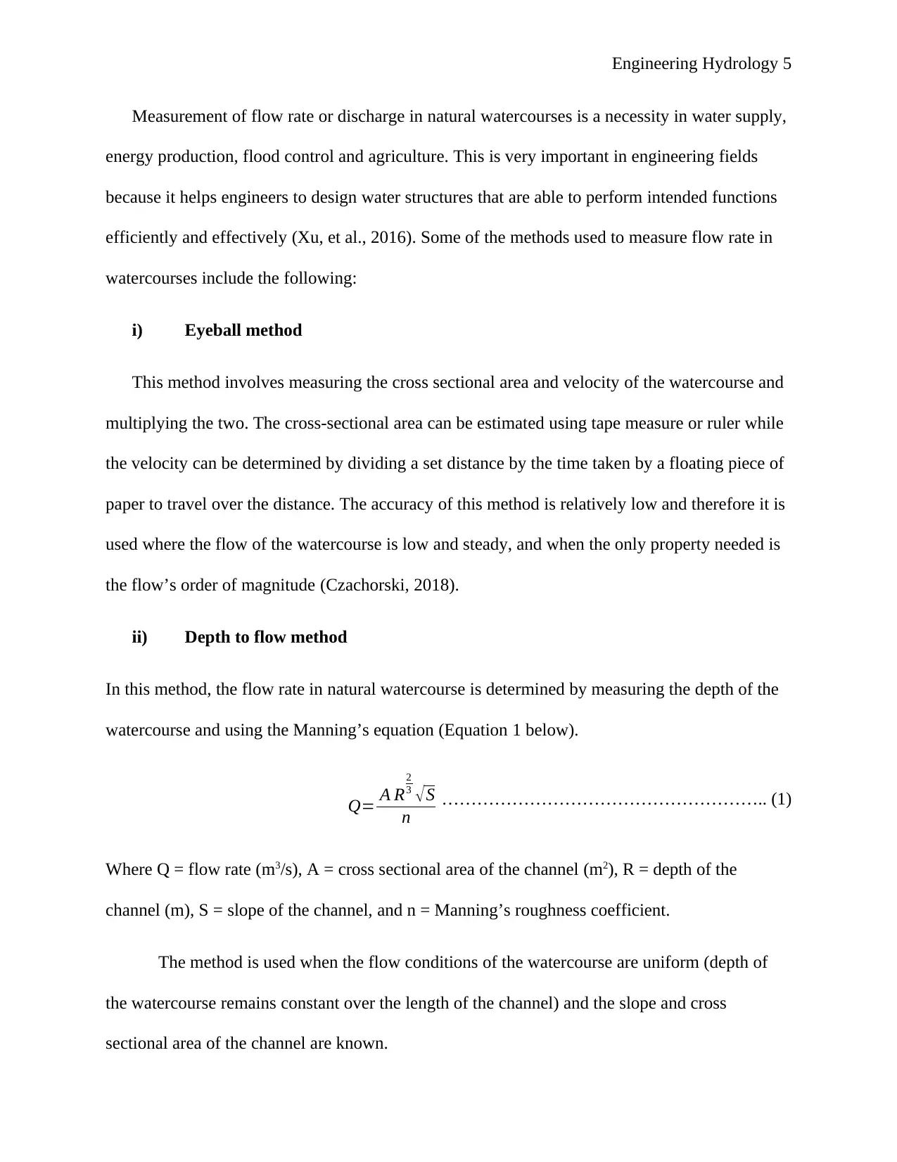
In this method, the flow rate in natural watercourse is determined by measuring the depth of the
watercourse and using the Manning’s equation (Equation 1 below).
Q= A R
2
3 √S
n
……………………………………………….. (1)
Where Q = flow rate (m3/s), A = cross sectional area of the channel (m2), R = depth of the
channel (m), S = slope of the channel, and n = Manning’s roughness coefficient.
The method is used when the flow conditions of the watercourse are uniform (depth of
the watercourse remains constant over the length of the channel) and the slope and cross
sectional area of the channel are known.
Measurement of flow rate or discharge in natural watercourses is a necessity in water supply,
energy production, flood control and agriculture. This is very important in engineering fields
because it helps engineers to design water structures that are able to perform intended functions
efficiently and effectively (Xu, et al., 2016). Some of the methods used to measure flow rate in
watercourses include the following:
i) Eyeball method
This method involves measuring the cross sectional area and velocity of the watercourse and
multiplying the two. The cross-sectional area can be estimated using tape measure or ruler while
the velocity can be determined by dividing a set distance by the time taken by a floating piece of
paper to travel over the distance. The accuracy of this method is relatively low and therefore it is
used where the flow of the watercourse is low and steady, and when the only property needed is
the flow’s order of magnitude (Czachorski, 2018).
ii) Depth to flow method
In this method, the flow rate in natural watercourse is determined by measuring the depth of the
watercourse and using the Manning’s equation (Equation 1 below).
Q= A R
2
3 √S
n
……………………………………………….. (1)
Where Q = flow rate (m3/s), A = cross sectional area of the channel (m2), R = depth of the
channel (m), S = slope of the channel, and n = Manning’s roughness coefficient.
The method is used when the flow conditions of the watercourse are uniform (depth of
the watercourse remains constant over the length of the channel) and the slope and cross
sectional area of the channel are known.
Engineering Hydrology 6
iii) Immersed current meter
This is a conventional method for measuring flow rate in natural watercourses. In this
method, a current meter is immersed at different points across the watercourse to measure and
record the mean flow velocity of the section (National Environmental Monitoring Standards
(NEMS) Group, 2013). The mean flow velocity is the used to calculate the flow rate using
computational methods (i.e. by multiplying it with the cross-sectional area of the flow at each of
the sections). The flow rate is determined by finding the average of the products in the selected
sections of the watercourse. This is a simple and reliable method of measuring flow rate in
natural water courses and is mainly used for measuring low flow rate. However, it also becomes
difficult to measure flow rate when the water depth is not enough for immersion of the current
meter or when the velocity of the flow is below the minimum required by the meter's setting. Use
of immersed current meters is also hampered by turbulence.
iv) Surface velocity area method
This method is used to measure flow rate in natural watercourses by using surface devices to
determine the velocity if the flow, which is then multiplied by the cross sectional area of the
open channel (Alvisi, et al., 2014). The velocity of the flow can be measured using
electromagnetic, mechanical or acoustic open channel flow meters (Almedia & Souza, 2017).
The velocity of the watercourse can be measured from the surface sing close range
photogrammetry, total stations or even remotely piloted aircraft systems (also known as drones)
(Tauro, et al., 2015); (Bolognesi, et al., 2017). This method is mainly used in areas where it is
difficult to access the watercourse in order to measure the flow velocity. It is also suitable for use
in watercourses with uniform flow conditions and cross sectional area.
⊘ This is a preview!⊘
Do you want full access?
Subscribe today to unlock all pages.
Trusted by 1+ million students worldwide
Engineering Hydrology 7
v) Artificial tracing method
This method involves use of tracers such as chemical tracers, radioactive tracers and
fluorescent tracers. Chemical tracers can be used in small and wide watercourses but are most
suitable for use in small watercourses because they are easy to handle, low cost, provide
satisfactory results and have low impact on the watercourse. In this method, a tracer of known
concentration is released instantaneously at the release section of the watercourse then its
concentration is determined in a downstream measuring section (Christiansen, 2009). The flow
rate is then calculated using computation method where the inputs are the concentration of the
tracer at the release and measuring sections, the volume of the water between the two sections,
and the time taken by the tracer to travel between the two sections. The choice of most suitable
tracer is determined by: chemical water characteristics, distance between release and measuring
section, type of suspended sediment in the watercourse, type of flow, watercourse’s hydrological
characteristics (Rowinski & Chrzanowski, 2011), and trace measurement equipment’s sensitivity
(Tazioli, 2011). This method is suitable for use when measuring very high flow rate in a
watercourse, such as during flood events. However, the method is not very effective when the
water is turbid because in such a case, the tracers may be easily absorbed by the suspended
sediments.
vi) Primary device method
This method measures the flow rate in natural watercourses using hydraulic structures such
as a weir, flume or dam, which enables flow rate measurement by measuring depth (Open
Channel Flow, (n.d.)). The measured depth can then be converted to a flow rate using a rating
curve equation or computational formula. Primary devices are designed to force the flow of the
watercourse to pass through critical depth (Goel, et al., 2015), which corresponds to a single flow
Paraphrase This Document
Need a fresh take? Get an instant paraphrase of this document with our AI Paraphraser
Engineering Hydrology 8
rate (Samani, 2017). These devices are easy to use and maintain. The method is very accurate
and mainly used to measure flow rate in watercourses that have these primary devices. However,
primary devices can cause backwater and head loss in the system thus reducing the accuracy of
the flow rate measurement.
The main factors determining the choice of suitable method for measuring flow rate in natural
watercourses are type of flow and conditions of the watercourse.
c) How to separate base flow from the hydrograph of a stream’s discharge
There are various methods that can be used to separate base flow from the hydrograph of a
stream’s discharge. In this case, it is assumed that the hydrograph (a curve showing the
relationship between discharge of the stream and time) has already been drawn. The hydrograph
comprises of two limbs: rising limb and falling limb. Rising limb is the curve between the start
of runoff and peak discharge whereas the falling limb is the curve between the peak point and
end of storm flow. The method used to separate base flow from the hydrograph in this scenario is
straight line method. This is the simplest method for separating the base flow from a hydrograph
and is only suitable for individual storm events. The first step is to identify the time when direct
runoff started on the hydrograph. This point is easy to locate because it is basically the point
where the hydrograph starts rising sharply and is determined by simply inspecting the
hydrograph visually. The rising limb is also referred to as the concentration curve and it is the
ascending part of the hydrograph. (Riya, (n.d.)) The point corresponding to this time is marked
on the hydrograph (point A in Figure 2 below).
Engineering Hydrology 9
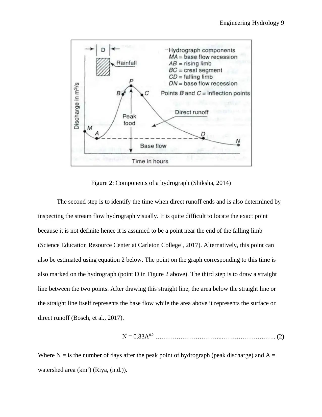
Figure 2: Components of a hydrograph (Shiksha, 2014)
The second step is to identify the time when direct runoff ends and is also determined by
inspecting the stream flow hydrograph visually. It is quite difficult to locate the exact point
because it is not definite hence it is assumed to be a point near the end of the falling limb
(Science Education Resource Center at Carleton College , 2017). Alternatively, this point can
also be estimated using equation 2 below. The point on the graph corresponding to this time is
also marked on the hydrograph (point D in Figure 2 above). The third step is to draw a straight
line between the two points. After drawing this straight line, the area below the straight line or
the straight line itself represents the base flow while the area above it represents the surface or
direct runoff (Bosch, et al., 2017).
N = 0.83A0.2 …………………………..…………………….. (2)
Where N = is the number of days after the peak point of hydrograph (peak discharge) and A =
watershed area (km2) (Riya, (n.d.)).
⊘ This is a preview!⊘
Do you want full access?
Subscribe today to unlock all pages.
Trusted by 1+ million students worldwide
Engineering Hydrology 10
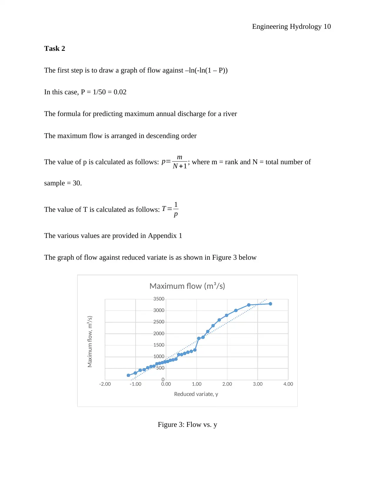
Task 2
The first step is to draw a graph of flow against –ln(-ln(1 – P))
In this case, P = 1/50 = 0.02
The formula for predicting maximum annual discharge for a river
The maximum flow is arranged in descending order
The value of p is calculated as follows: p= m
N +1 ; where m = rank and N = total number of
sample = 30.
The value of T is calculated as follows: T = 1
p
The various values are provided in Appendix 1
The graph of flow against reduced variate is as shown in Figure 3 below
-2.00 -1.00 0.00 1.00 2.00 3.00 4.00
0
500
1000
1500
2000
2500
3000
3500
Maximum flow (m³/s)
Reduced variate, y
Maximum flow, m³/s)
Figure 3: Flow vs. y
Paraphrase This Document
Need a fresh take? Get an instant paraphrase of this document with our AI Paraphraser
Engineering Hydrology 11
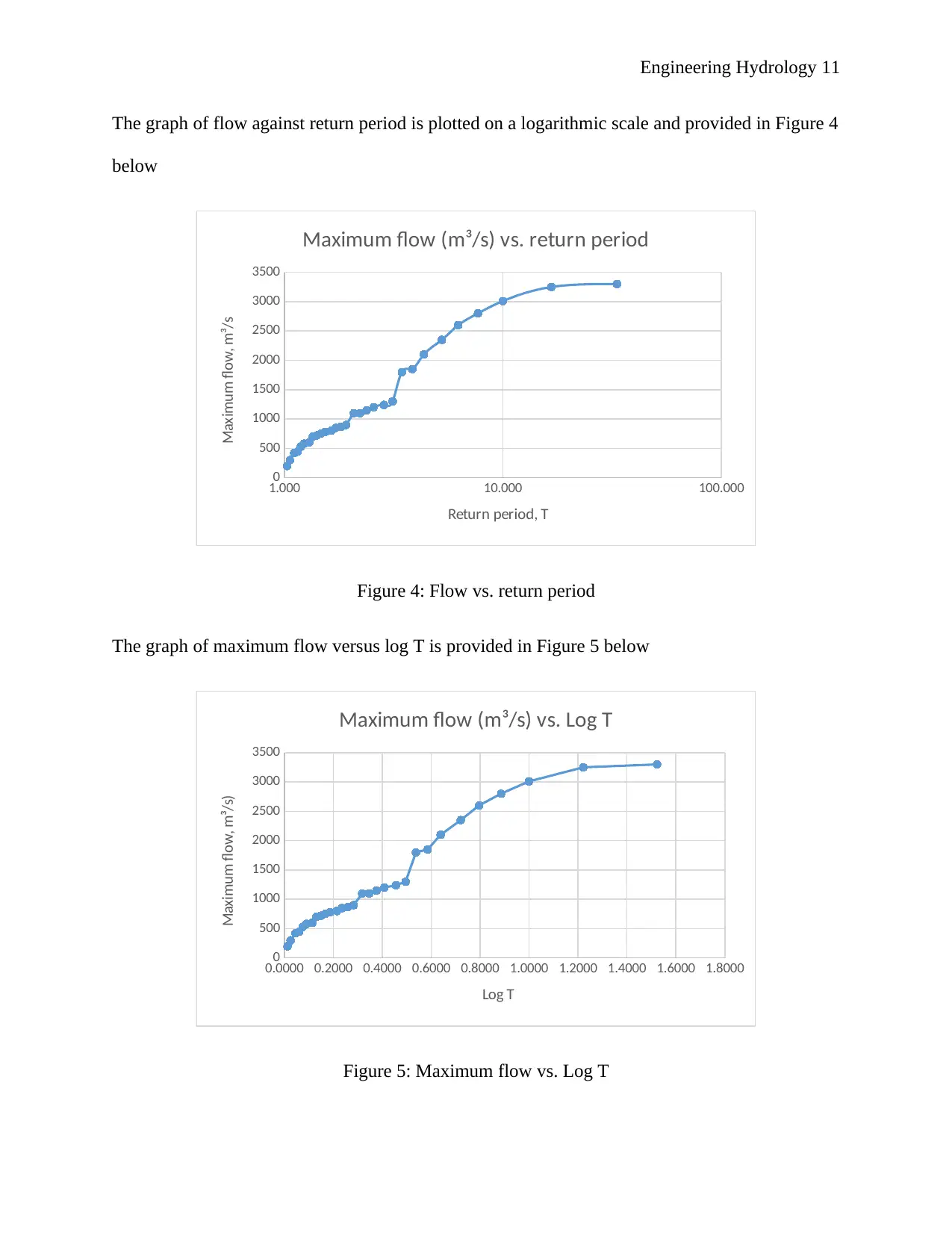
The graph of flow against return period is plotted on a logarithmic scale and provided in Figure 4
below
1.000 10.000 100.000
0
500
1000
1500
2000
2500
3000
3500
Maximum flow (m³/s) vs. return period
Return period, T
Maximum flow, m³/s
Figure 4: Flow vs. return period
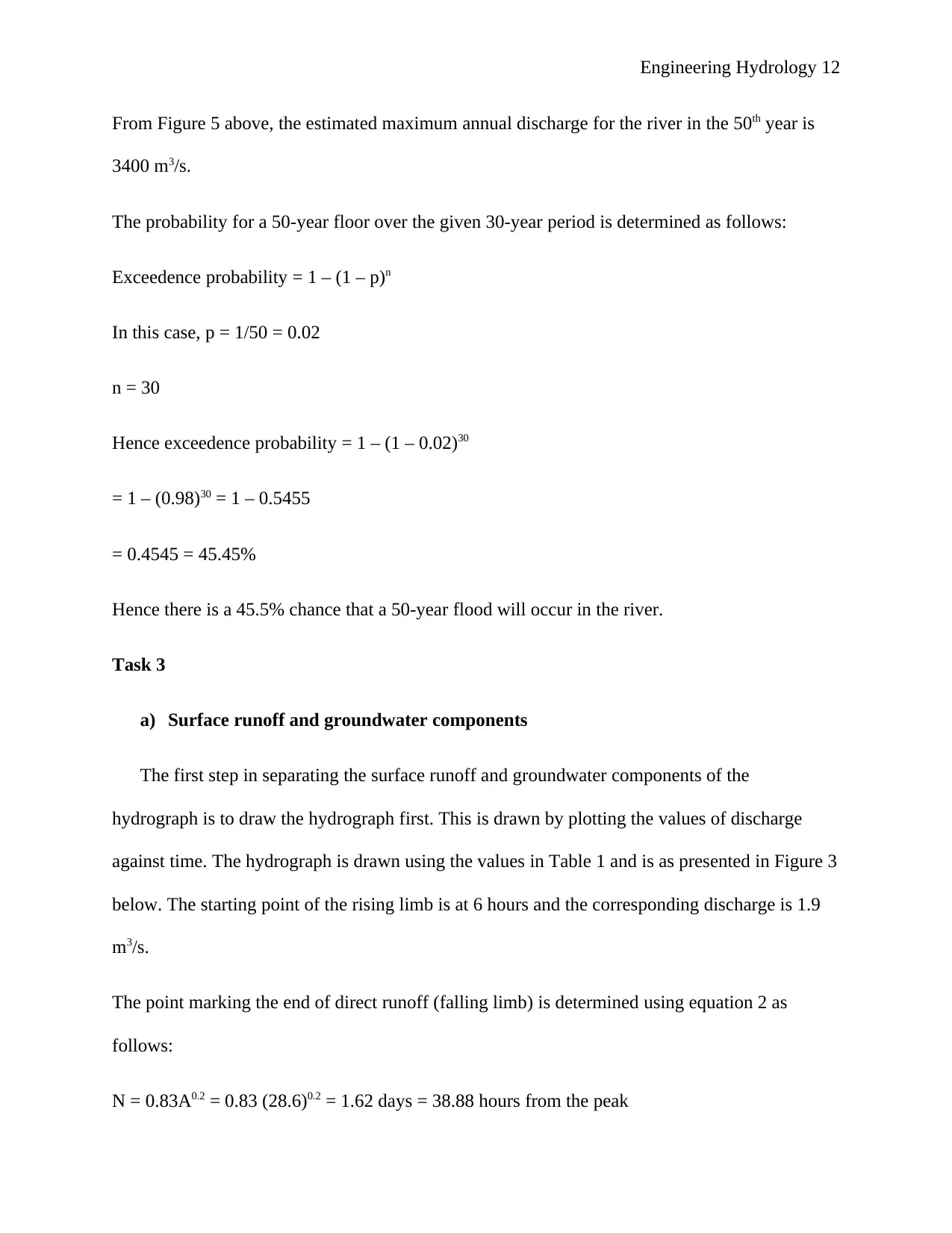
The graph of maximum flow versus log T is provided in Figure 5 below
0.0000 0.2000 0.4000 0.6000 0.8000 1.0000 1.2000 1.4000 1.6000 1.8000
0
500
1000
1500
2000
2500
3000
3500
Maximum flow (m³/s) vs. Log T
Log T
Maximum flow, m³/s)
Figure 5: Maximum flow vs. Log T
The graph of flow against return period is plotted on a logarithmic scale and provided in Figure 4
below
1.000 10.000 100.000
0
500
1000
1500
2000
2500
3000
3500
Maximum flow (m³/s) vs. return period
Return period, T
Maximum flow, m³/s
Figure 4: Flow vs. return period
The graph of maximum flow versus log T is provided in Figure 5 below
0.0000 0.2000 0.4000 0.6000 0.8000 1.0000 1.2000 1.4000 1.6000 1.8000
0
500
1000
1500
2000
2500
3000
3500
Maximum flow (m³/s) vs. Log T
Log T
Maximum flow, m³/s)
Figure 5: Maximum flow vs. Log T
Engineering Hydrology 12
From Figure 5 above, the estimated maximum annual discharge for the river in the 50th year is
3400 m3/s.
The probability for a 50-year floor over the given 30-year period is determined as follows:
Exceedence probability = 1 – (1 – p)n
In this case, p = 1/50 = 0.02
n = 30
Hence exceedence probability = 1 – (1 – 0.02)30
= 1 – (0.98)30 = 1 – 0.5455
= 0.4545 = 45.45%
Hence there is a 45.5% chance that a 50-year flood will occur in the river.
Task 3
a) Surface runoff and groundwater components
The first step in separating the surface runoff and groundwater components of the
hydrograph is to draw the hydrograph first. This is drawn by plotting the values of discharge
against time. The hydrograph is drawn using the values in Table 1 and is as presented in Figure 3
below. The starting point of the rising limb is at 6 hours and the corresponding discharge is 1.9
m3/s.
The point marking the end of direct runoff (falling limb) is determined using equation 2 as
follows:
N = 0.83A0.2 = 0.83 (28.6)0.2 = 1.62 days = 38.88 hours from the peak
⊘ This is a preview!⊘
Do you want full access?
Subscribe today to unlock all pages.
Trusted by 1+ million students worldwide
1 out of 22
Related Documents


Your All-in-One AI-Powered Toolkit for Academic Success.
+13062052269
info@desklib.com
Available 24*7 on WhatsApp / Email
![[object Object]](/_next/static/media/star-bottom.7253800d.svg)
Unlock your academic potential
Copyright © 2020–2026 A2Z Services. All Rights Reserved. Developed and managed by ZUCOL.