Engineering Mathematics MATLAB Assignment Solution, 2018-19

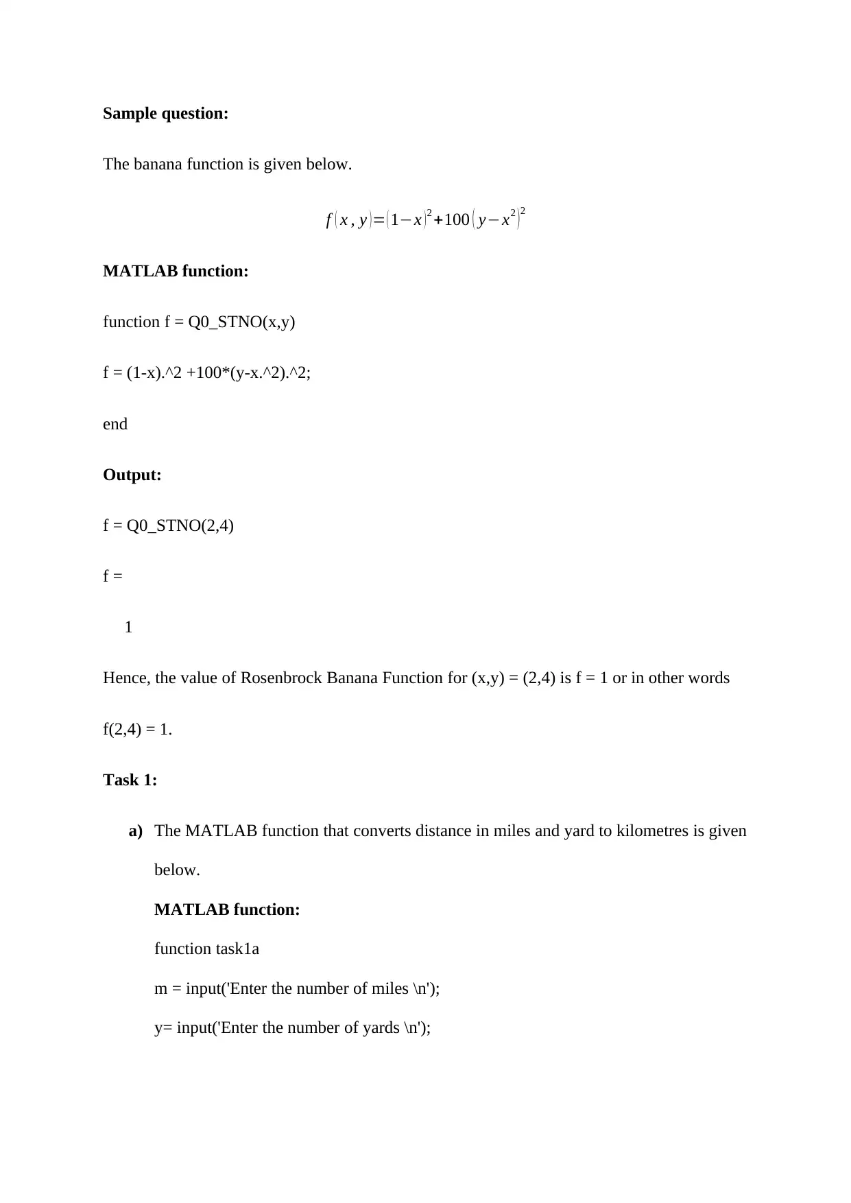
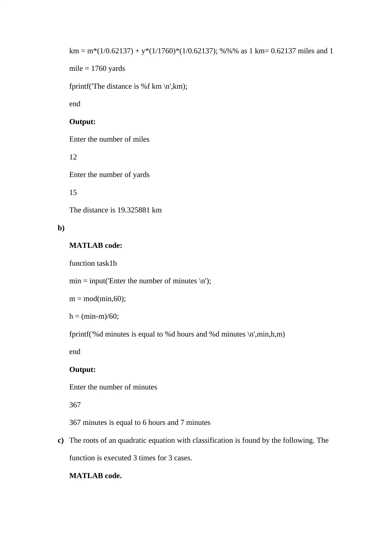
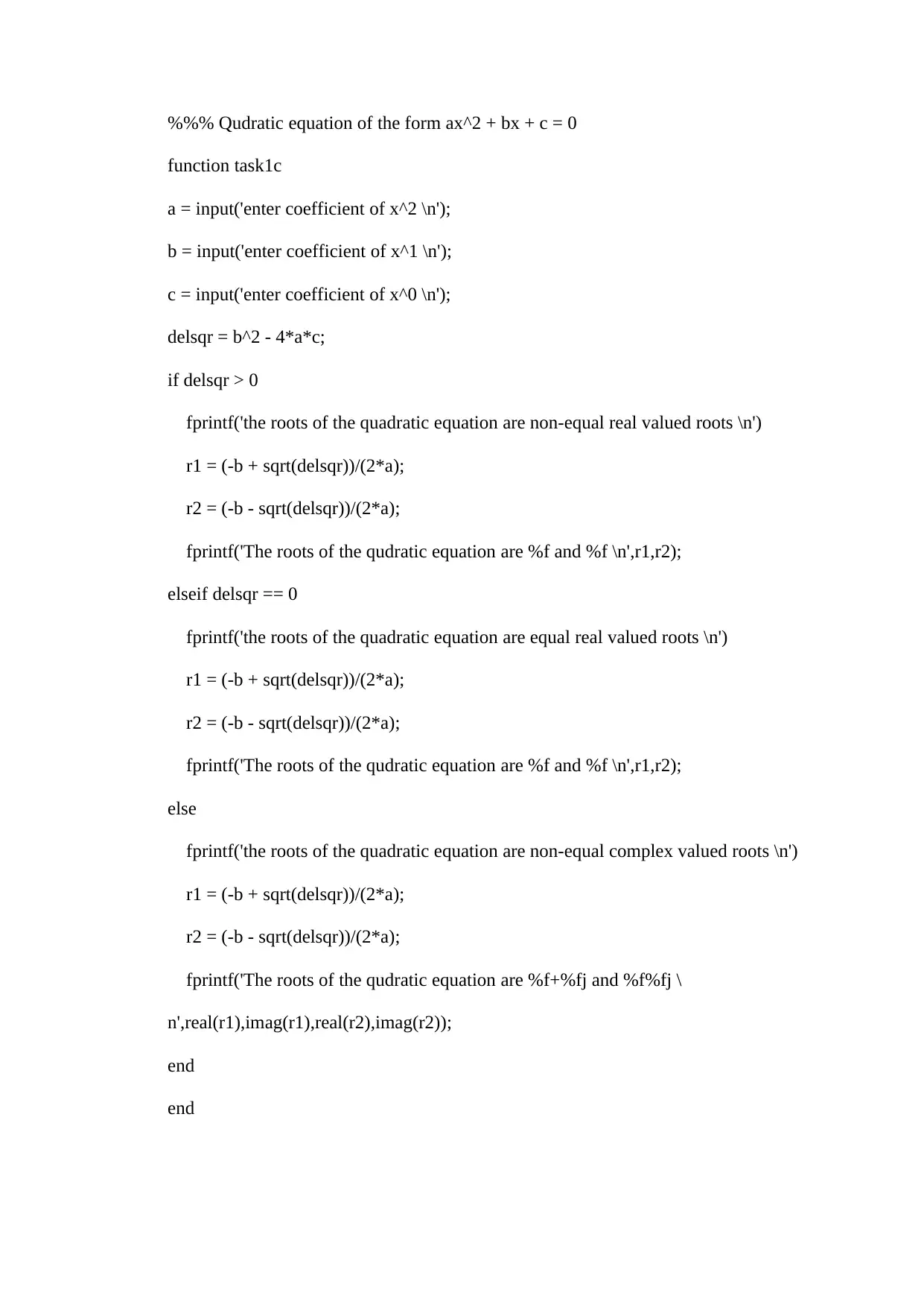
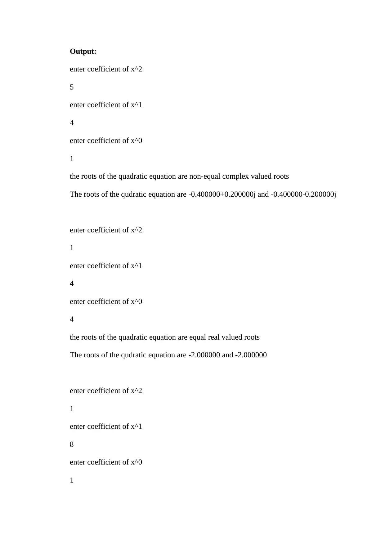
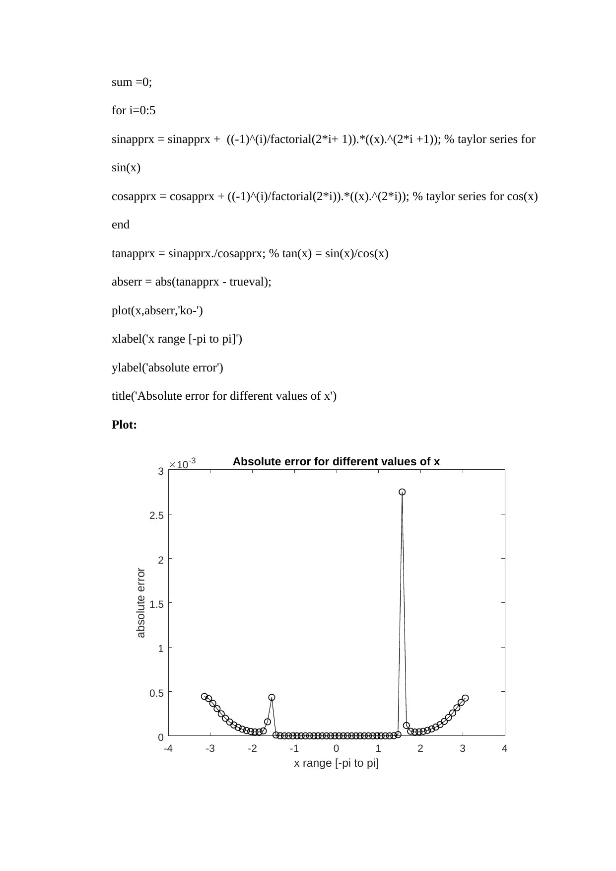
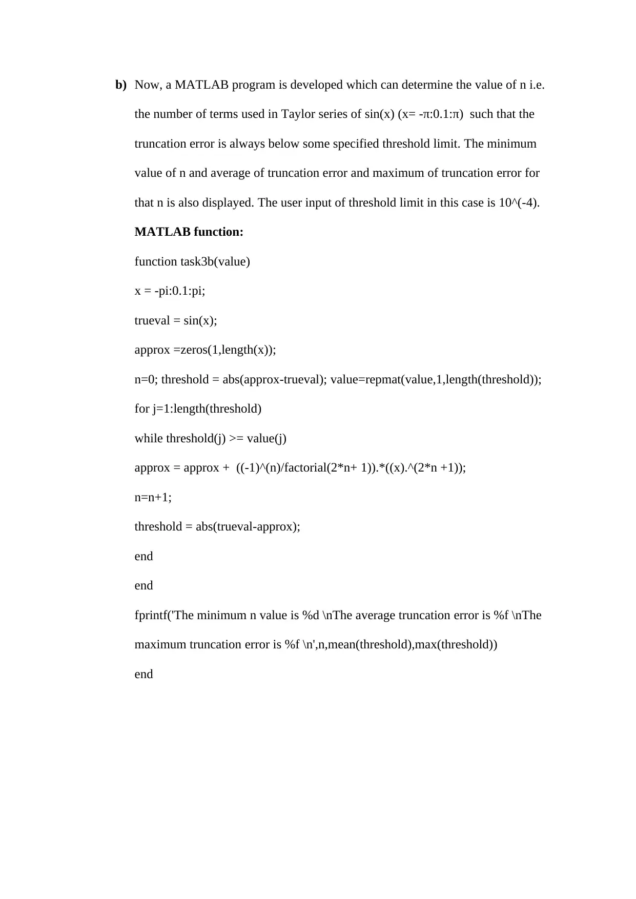
This document presents a comprehensive MATLAB assignment solution for an Engineering Mathematics course. The assignment is divided into three tasks. Task 1 focuses on creating MATLAB functions to convert miles and yards to kilometers, convert minutes to hours and minutes, and solve quadratic equations, classifying the roots. Task 2 involves analyzing braking distances at different speeds, calculating correlation coefficients, and generating a regression line with a scatter plot. Task 3 explores Taylor series applications, including calculating sin(π/5) using a Taylor series with varying terms and plotting the percentage error. The assignment also includes a program to determine the number of terms needed for a Taylor series of sin(x) to achieve a specified truncation error threshold, displaying the minimum number of terms, average, and maximum truncation errors.

Sample question:
The banana function is given below.
f ( x , y ) = ( 1−x ) 2 +100 ( y−x2 ) 2
MATLAB function:
function f = Q0_STNO(x,y)
f = (1-x).^2 +100*(y-x.^2).^2;
end
Output:
f = Q0_STNO(2,4)
f =
1
Hence, the value of Rosenbrock Banana Function for (x,y) = (2,4) is f = 1 or in other words
f(2,4) = 1.
Task 1:
a) The MATLAB function that converts distance in miles and yard to kilometres is given
below.
MATLAB function:
function task1a
m = input('Enter the number of miles \n');
y= input('Enter the number of yards \n');

km = m*(1/0.62137) + y*(1/1760)*(1/0.62137); %%% as 1 km= 0.62137 miles and 1
mile = 1760 yards
fprintf('The distance is %f km \n',km);
end
Output:
Enter the number of miles
12
Enter the number of yards
15
The distance is 19.325881 km
b)
MATLAB code:
function task1b
min = input('Enter the number of minutes \n');
m = mod(min,60);
h = (min-m)/60;
fprintf('%d minutes is equal to %d hours and %d minutes \n',min,h,m)
end
Output:
Enter the number of minutes
367
367 minutes is equal to 6 hours and 7 minutes
c) The roots of an quadratic equation with classification is found by the following. The
function is executed 3 times for 3 cases.
MATLAB code.

%%% Qudratic equation of the form ax^2 + bx + c = 0
function task1c
a = input('enter coefficient of x^2 \n');
b = input('enter coefficient of x^1 \n');
c = input('enter coefficient of x^0 \n');
delsqr = b^2 - 4*a*c;
if delsqr > 0
fprintf('the roots of the quadratic equation are non-equal real valued roots \n')
r1 = (-b + sqrt(delsqr))/(2*a);
r2 = (-b - sqrt(delsqr))/(2*a);
fprintf('The roots of the qudratic equation are %f and %f \n',r1,r2);
elseif delsqr == 0
fprintf('the roots of the quadratic equation are equal real valued roots \n')
r1 = (-b + sqrt(delsqr))/(2*a);
r2 = (-b - sqrt(delsqr))/(2*a);
fprintf('The roots of the qudratic equation are %f and %f \n',r1,r2);
else
fprintf('the roots of the quadratic equation are non-equal complex valued roots \n')
r1 = (-b + sqrt(delsqr))/(2*a);
r2 = (-b - sqrt(delsqr))/(2*a);
fprintf('The roots of the qudratic equation are %f+%fj and %f%fj \
n',real(r1),imag(r1),real(r2),imag(r2));
end
end

Output:
enter coefficient of x^2
5
enter coefficient of x^1
4
enter coefficient of x^0
1
the roots of the quadratic equation are non-equal complex valued roots
The roots of the qudratic equation are -0.400000+0.200000j and -0.400000-0.200000j
enter coefficient of x^2
1
enter coefficient of x^1
4
enter coefficient of x^0
4
the roots of the quadratic equation are equal real valued roots
The roots of the qudratic equation are -2.000000 and -2.000000
enter coefficient of x^2
1
enter coefficient of x^1
8
enter coefficient of x^0
1

the roots of the quadratic equation are non-equal real valued roots
The roots of the qudratic equation are -0.127017 and -7.872983
Task 2:
In this task the speed(in km/hr) is used as the independent variable and the total
braking distance is used as dependent variable.
Total braking distance = Thinking distance + braking distance = average thinking
time*(speed) + braking distance.
The braking distance (in m) is given for 6 different speeds (km/hr) in the question.
MATLAB code:
speed = [50 70 100 120 145 200]; % speed data
n= length(speed);
brake = [5 12.3 21 32.9 47.6 84.7]; % braking distance data
think = 1.8*(5/18).*speed; % Thinking distance. 1 km/hr = (5/18) m/sec.
tdist = think + brake; % total distance = branking distance + thinking distance
R = (n*sum(tdist.*speed) - sum(tdist)*sum(speed))/sqrt((n*sum(tdist.^2) -
(sum(tdist))^2)*(n*sum(speed.^2) - sum(speed)^2)); %% correleation coeffcient
calculation
a1 = R*((std(tdist)/std(speed))); % a1 = R*(sy/sx)
a0 = mean(tdist) - a1*mean(speed); % a0 = mean(y) - a1*mean(x)
fprintf('The coeffcient a0 = %f, coeffcient a1=%f and coefficient of determination
R^2 = %f \n',a0,a1,R^2)
y = repmat(a0,1,length(speed)) + a1.*speed; % least square regression line y = a0+
a1*x
scatter(speed,tdist)
hold on

plot(speed,y)
title('Scatter plot and fitted regression line')
xlabel('Speed in Km/hr')
ylabel('total braking distance in meters')
Output:
50 100 150 200
Speed in Km/hr
20
40
60
80
100
120
140
160
180
200
total braking distance in meters
Scatter plot and fitted regression line
The coefficient a0 = -26.740353, coefficient a1=1.031302 and coefficient of
determination R^2 = 0.992956
Hence, the regression line is y = -26.74 + 1.03*x and R^2 = 99.296%.
Where, y = total braking distance in meters.
x= speed in km/hr.
Task 3:
a)

i) The MATLAB function for calculating the value of sin(π/5) by using its
Taylor series of 1 to 6 terms( i.e. by using n=0 term, sum of n=0 and n=1
terms,…, sum of n=0 to n=5th terms) is given below. Additionally, the
percentage error from the true value of sin(π/5) (calculated using MATLAB
built in sin(x)) for each of the 6 cases is plotted w.r.t number of terms used.
Taylor series of sin(x )=∑
n=0
∞ (−1 )n x2 n +1
( 2 n+1 ) !
MATLAB function:
x = pi/5;
trueval = sin(x);
approx =0;
for i=0:5
approx(i+2) = approx(i+1) + (-1)^(i)*(x)^(2*i +1)/factorial(2*i+ 1);
end
for i =1:7
perror(i) = ((abs(trueval - approx(i)))/trueval)*100;
end
n =1:6;
plot(n,perror(2:end),'bo-')
title('Number of terms used in Taylor series vs percentage error')
xlabel('Number of terms used in Taylor series')
ylabel('Percentage error')
Plot:

1 1.5 2 2.5 3 3.5 4 4.5 5 5.5 6
Number of terms used in Taylor series
0
1
2
3
4
5
6
7
Percentage error
Number of terms used in Taylor series vs percentage error
The true value of sin(π/5) is found as 0.5878 and percentage error becomes zero
when using 4 or more terms.
ii) The MATLAB program for calculating tan(x) for x= -π:0.1:π by using Taylor
series is given below. The Taylor series with sum of 1st six terms of cos(x) and
sin(x) are used for generating Taylor series of tan(x).
cos (x)=∑
n=0
∞ (−1 )n x2 n
( 2 n ) !
tan ( x )= sin ( x )
cos ( x )
MATLAB code:
x = -pi:0.1:pi;
trueval = tan(x);
sinapprx = zeros(1,length(x));
cosapprx = zeros(1,length(x));

sum =0;
for i=0:5
sinapprx = sinapprx + ((-1)^(i)/factorial(2*i+ 1)).*((x).^(2*i +1)); % taylor series for
sin(x)
cosapprx = cosapprx + ((-1)^(i)/factorial(2*i)).*((x).^(2*i)); % taylor series for cos(x)
end
tanapprx = sinapprx./cosapprx; % tan(x) = sin(x)/cos(x)
abserr = abs(tanapprx - trueval);
plot(x,abserr,'ko-')
xlabel('x range [-pi to pi]')
ylabel('absolute error')
title('Absolute error for different values of x')
Plot:
-4 -3 -2 -1 0 1 2 3 4
x range [-pi to pi]
0
0.5
1
1.5
2
2.5
3
absolute error
10-3 Absolute error for different values of x

b) Now, a MATLAB program is developed which can determine the value of n i.e.
the number of terms used in Taylor series of sin(x) (x= -π:0.1:π) such that the
truncation error is always below some specified threshold limit. The minimum
value of n and average of truncation error and maximum of truncation error for
that n is also displayed. The user input of threshold limit in this case is 10^(-4).
MATLAB function:
function task3b(value)
x = -pi:0.1:pi;
trueval = sin(x);
approx =zeros(1,length(x));
n=0; threshold = abs(approx-trueval); value=repmat(value,1,length(threshold));
for j=1:length(threshold)
while threshold(j) >= value(j)
approx = approx + ((-1)^(n)/factorial(2*n+ 1)).*((x).^(2*n +1));
n=n+1;
threshold = abs(trueval-approx);
end
end
fprintf('The minimum n value is %d \nThe average truncation error is %f \nThe
maximum truncation error is %f \n',n,mean(threshold),max(threshold))
end

Output:
task3b(1e-4)
The minimum n value is 7
The average truncation error is 0.000001
The maximum truncation error is 0.000021