Horizon Labs Internship: Engineering Mathematics Wave Equation Report
VerifiedAdded on  2023/01/20
|20
|2432
|67
Report
AI Summary
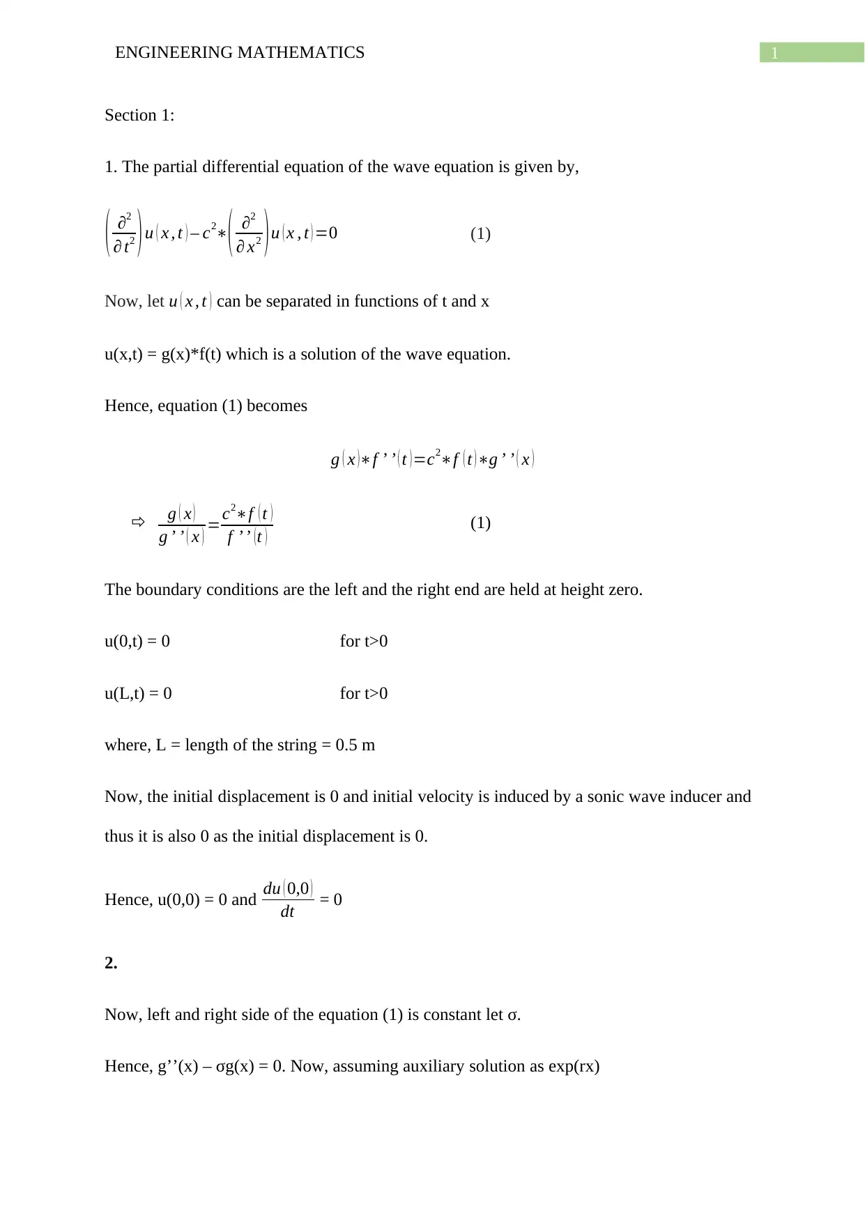
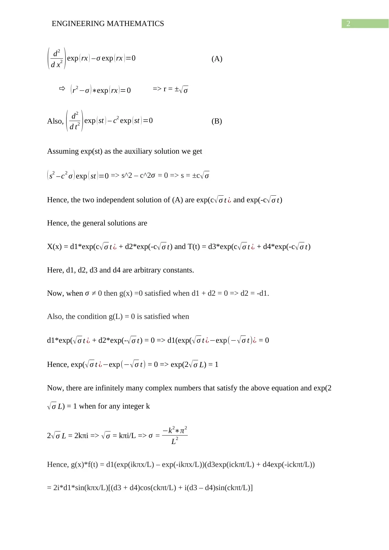
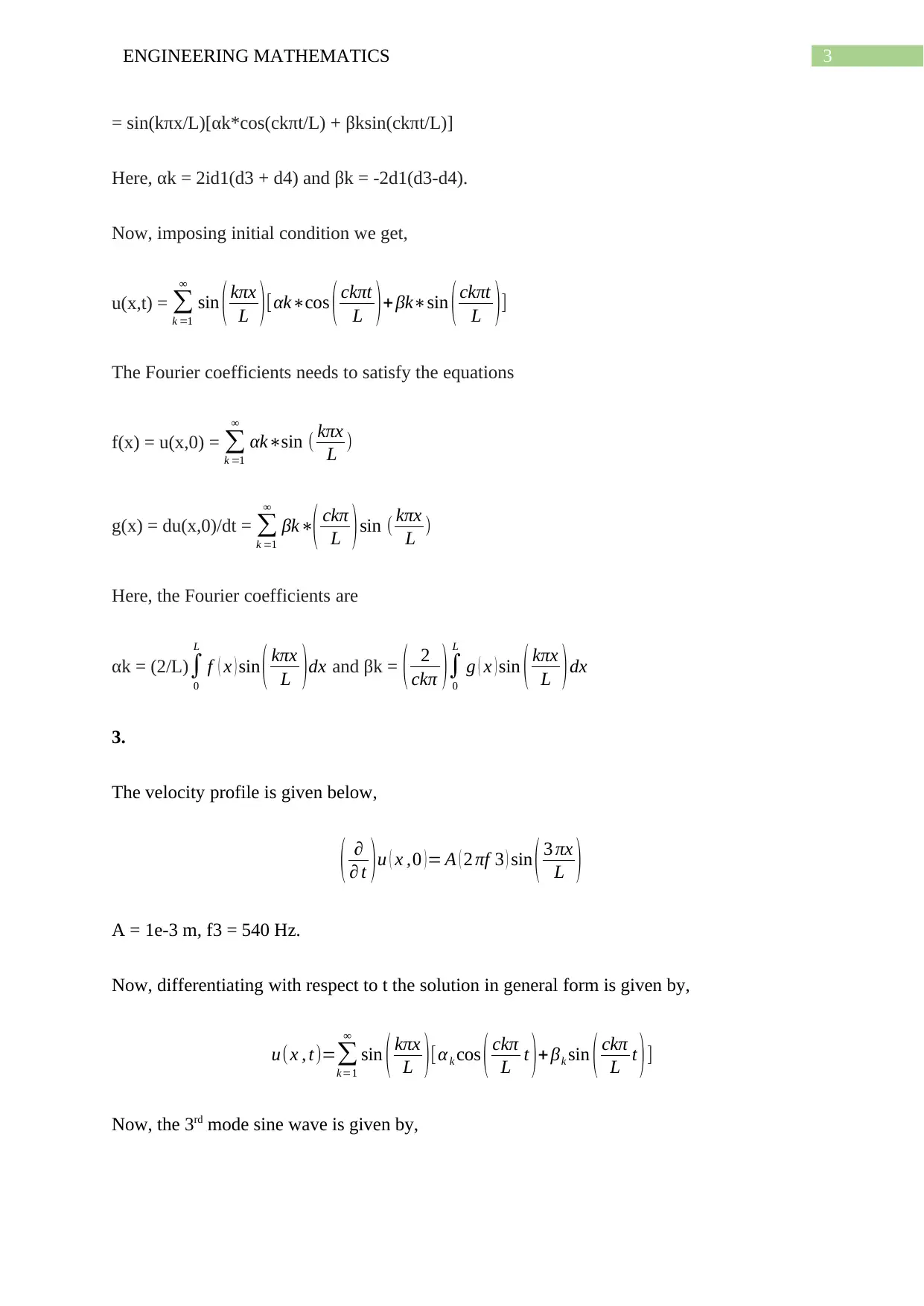
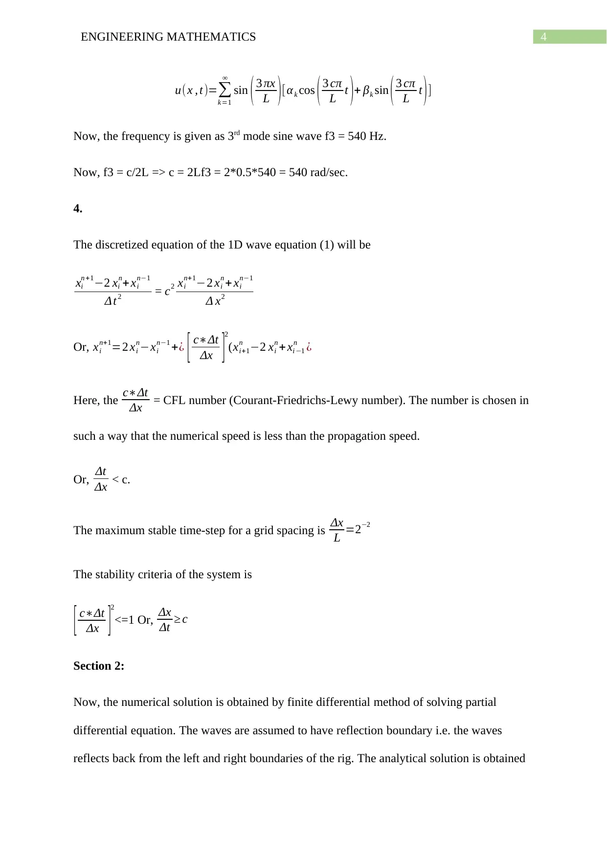
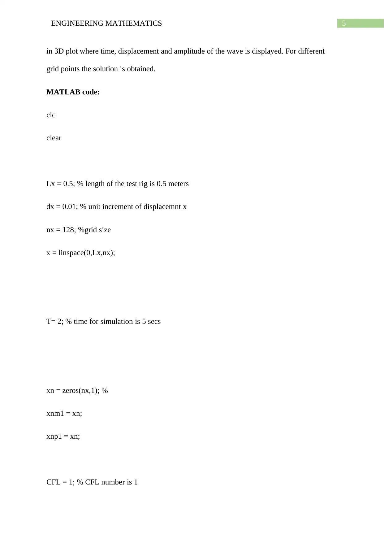
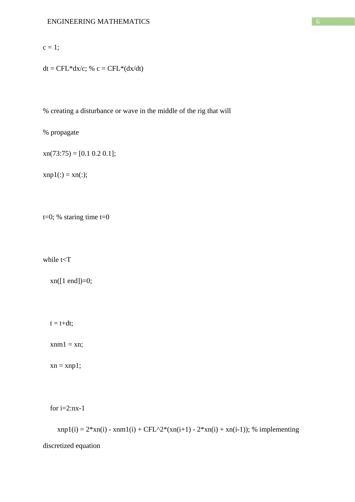
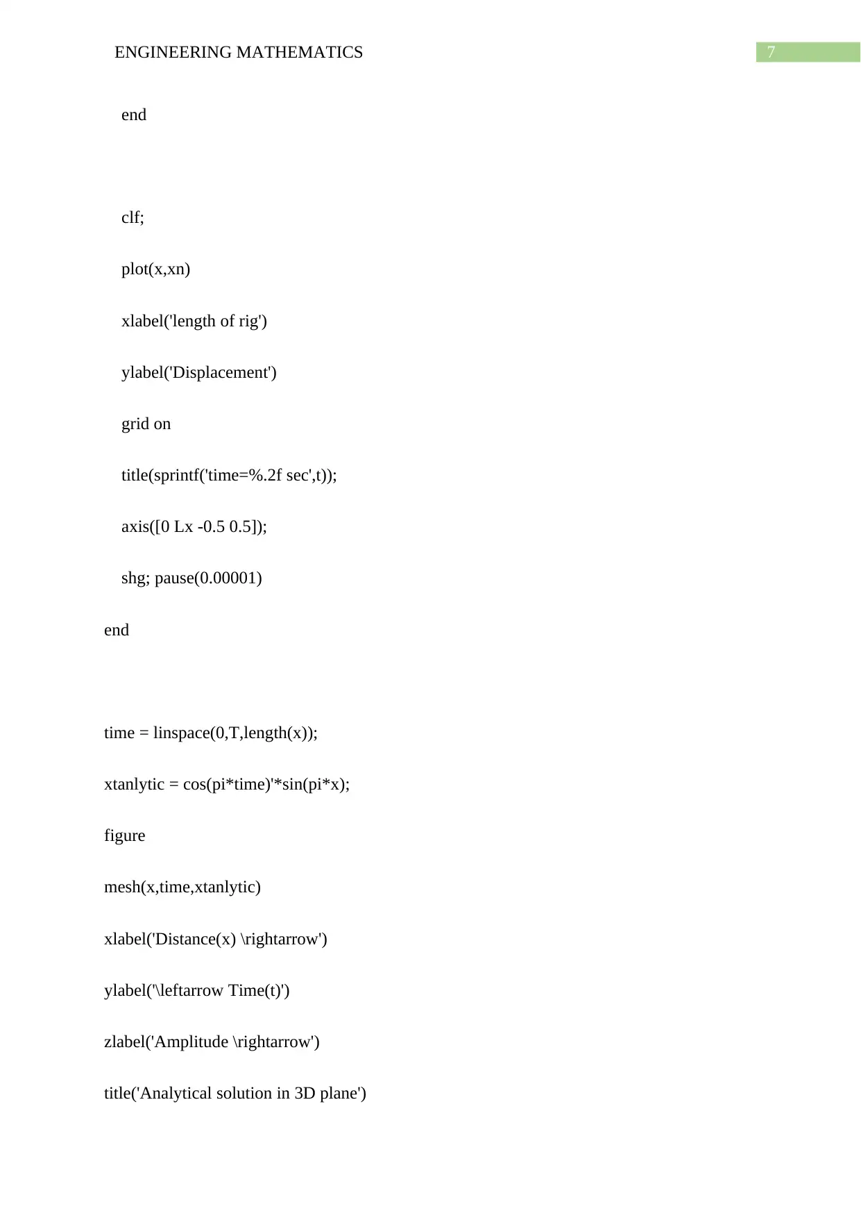
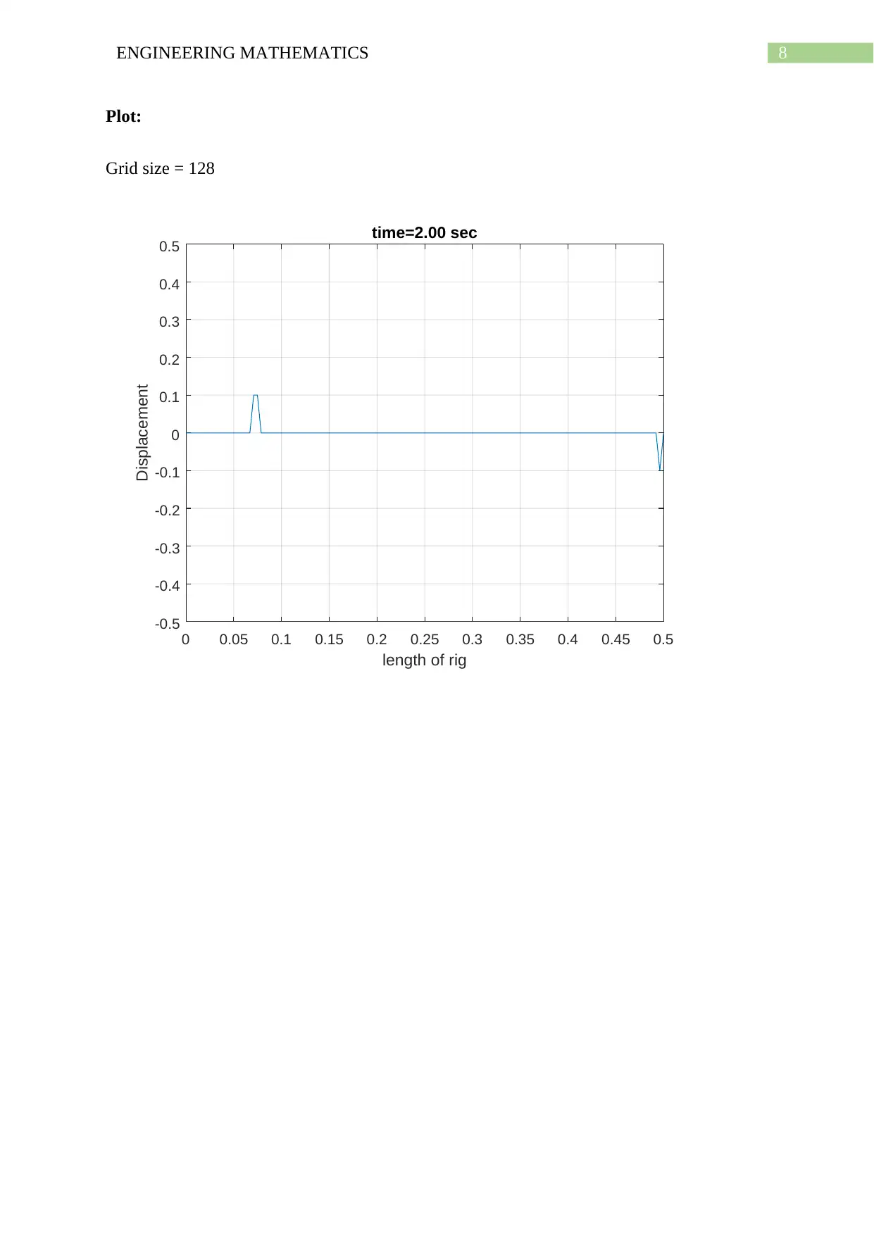
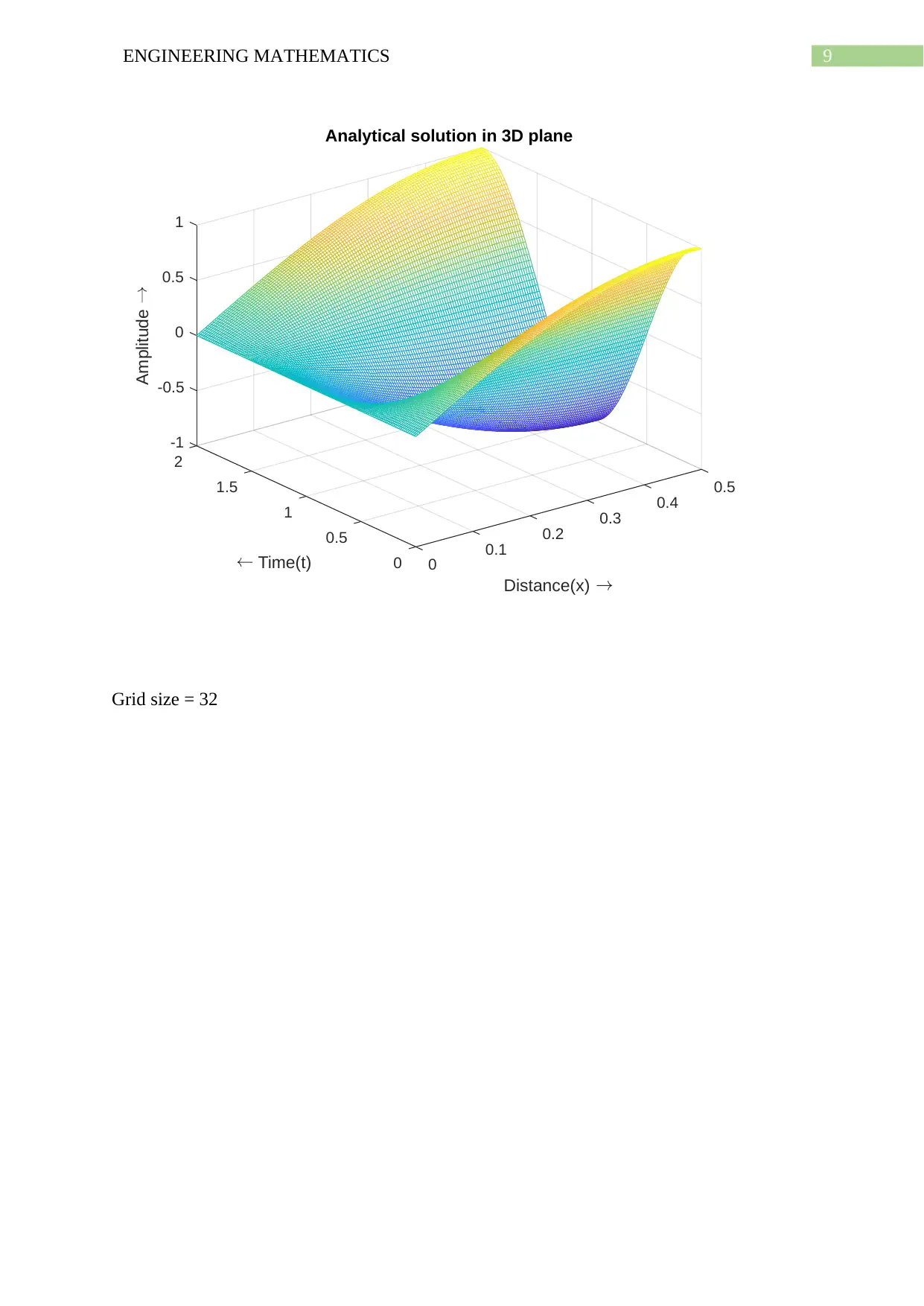
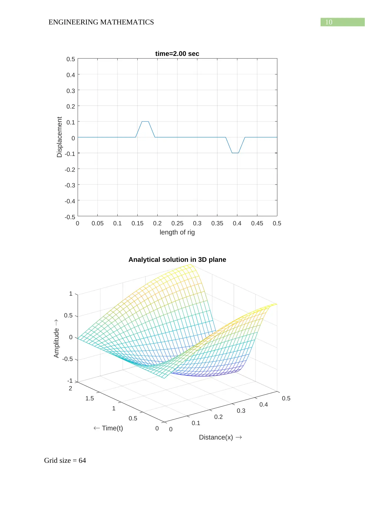
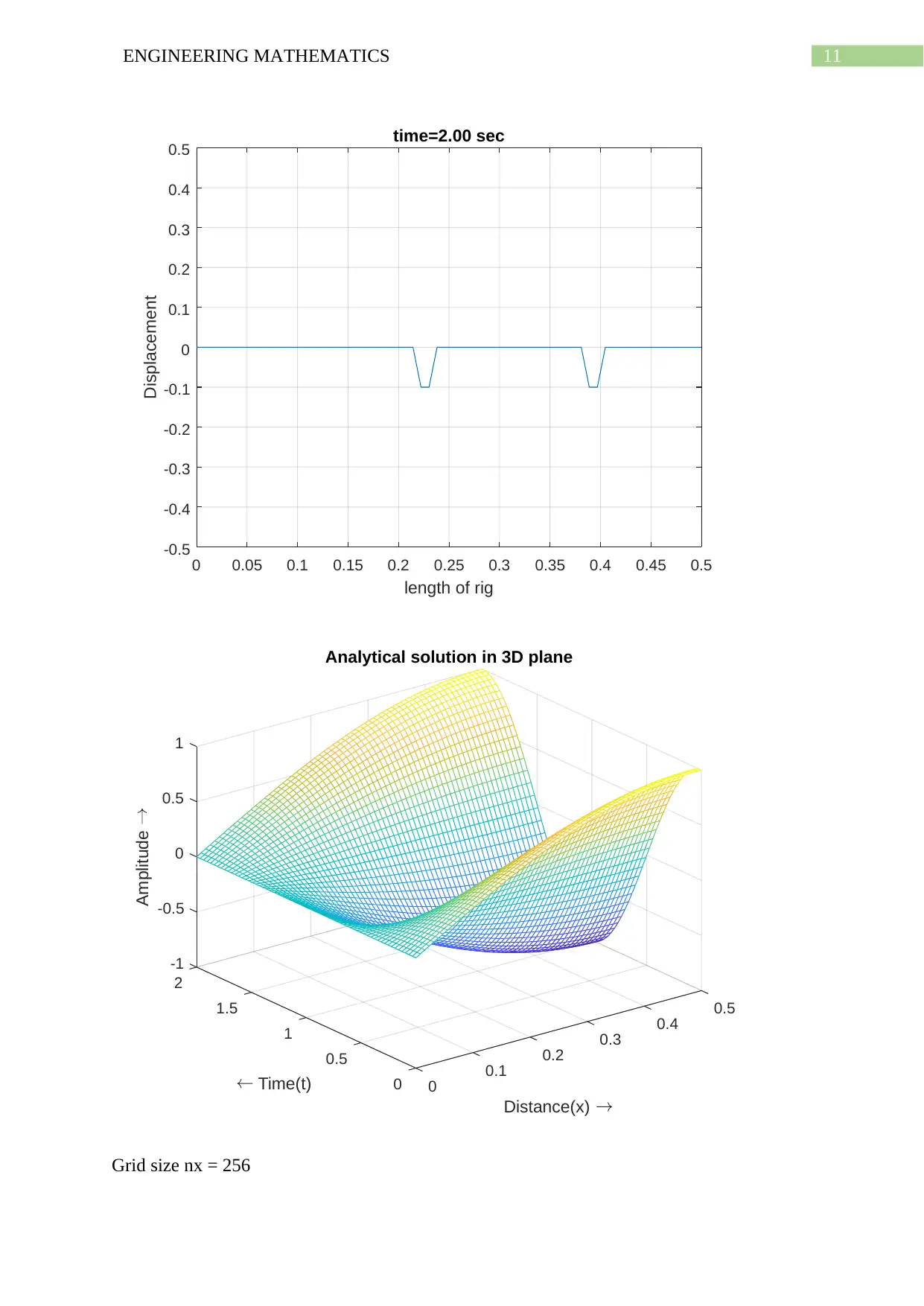
This report presents an analysis of the 1D wave equation, focusing on numerical solutions obtained through the finite difference method and MATLAB simulations. Section 1 formulates the wave equation, derives boundary conditions, and explores analytical solutions using separation of variables. Section 2 delves into numerical solutions, utilizing MATLAB code to simulate wave propagation and visualize results with varying grid sizes, comparing the numerical solution to an analytical solution. The report also investigates the effects of changing the grid size. Section 3 extends the analysis to include a forcing function, simulating the impact of a sonic wave inducer on the web. The report discusses the influence of the force amplitude and frequency on the wave behavior, providing graphical outputs for different parameter values.

Running head: ENGINEERING MATHEMATICS
ENGINEERING MATHEMATICS
Name of the Student
Name of the University
Author Note
ENGINEERING MATHEMATICS
Name of the Student
Name of the University
Author Note
Paraphrase This Document
Need a fresh take? Get an instant paraphrase of this document with our AI Paraphraser

1ENGINEERING MATHEMATICS
Section 1:
1. The partial differential equation of the wave equation is given by,
( ∂2
∂ t2 )u ( x , t ) – c2∗( ∂2
∂ x2 )u ( x , t ) =0 (1)
Now, let u ( x , t ) can be separated in functions of t and x
u(x,t) = g(x)*f(t) which is a solution of the wave equation.
Hence, equation (1) becomes
g ( x )∗f ’ ’ ( t )=c2∗f ( t )∗g ’ ’ ( x )
 g ( x )
g ’ ’ ( x ) =c2∗f ( t )
f ’’ ( t ) (1)
The boundary conditions are the left and the right end are held at height zero.
u(0,t) = 0 for t>0
u(L,t) = 0 for t>0
where, L = length of the string = 0.5 m
Now, the initial displacement is 0 and initial velocity is induced by a sonic wave inducer and
thus it is also 0 as the initial displacement is 0.
Hence, u(0,0) = 0 and du ( 0,0 )
dt = 0
2.
Now, left and right side of the equation (1) is constant let σ.
Hence, g’’(x) – σg(x) = 0. Now, assuming auxiliary solution as exp(rx)

2ENGINEERING MATHEMATICS
( d2
d x2 )exp ( rx ) – σ exp ( rx )=0 (A)
 ( r2 −σ )∗exp ( rx )=0 => r = ±√σ
Also, ( d2
d t2 ) exp ( st ) – c2 exp ( st ) =0 (B)
Assuming exp(st) as the auxiliary solution we get
( s2 – c2 σ ) exp ( st )=0 => s^2 – c^2σ = 0 => s = ±c√σ
Hence, the two independent solution of (A) are exp(c √ σ t ¿ and exp(-c√σ t)
Hence, the general solutions are
X(x) = d1*exp(c √ σ t ¿ + d2*exp(-c√σ t) and T(t) = d3*exp(c√ σ t ¿ + d4*exp(-c√σ t)
Here, d1, d2, d3 and d4 are arbitrary constants.
Now, when σ ≠0 then g(x) =0 satisfied when d1 + d2 = 0 => d2 = -d1.
Also, the condition g(L) = 0 is satisfied when
d1*exp( √σ t ¿ + d2*exp(- √ σ t) = 0 => d1(exp(√ σ t ¿−exp(− √ σ t)¿ = 0
Hence, exp(√ σ t ¿−exp(− √ σ t) = 0 => exp(2 √σ L) = 1
Now, there are infinitely many complex numbers that satisfy the above equation and exp(2
√ σ L) = 1 when for any integer k
2√ σ L = 2kπi => √σ = kπi/L => σ = −k2∗π2
L2
Hence, g(x)*f(t) = d1(exp(ikπx/L) – exp(-ikπx/L))(d3exp(ickπt/L) + d4exp(-ickπt/L))
= 2i*d1*sin(kπx/L)[(d3 + d4)cos(ckπt/L) + i(d3 – d4)sin(ckπt/L)]
⊘ This is a preview!⊘
Do you want full access?
Subscribe today to unlock all pages.

Trusted by 1+ million students worldwide

3ENGINEERING MATHEMATICS
= sin(kπx/L)[αk*cos(ckπt/L) + βksin(ckπt/L)]
Here, αk = 2id1(d3 + d4) and βk = -2d1(d3-d4).
Now, imposing initial condition we get,
u(x,t) = ∑
k =1
∞
sin ( kπx
L ) [αk∗cos ( ckπt
L ) + βk∗sin ( ckπt
L ) ]
The Fourier coefficients needs to satisfy the equations
f(x) = u(x,0) = ∑
k =1
∞
αk∗sin ( kπx
L )
g(x) = du(x,0)/dt = ∑
k =1
∞
βk∗( ckπ
L ) sin ( kπx
L )
Here, the Fourier coefficients are
αk = (2/L) ∫
0
L
f ( x ) sin ( kπx
L ) dx and βk = ( 2
ckπ )∫
0
L
g ( x ) sin ( kπx
L ) dx
3.
The velocity profile is given below,
( ∂
∂ t )u ( x ,0 )= A ( 2 πf 3 ) sin ( 3 πx
L )
A = 1e-3 m, f3 = 540 Hz.
Now, differentiating with respect to t the solution in general form is given by,
u(x , t)=∑
k=1
∞
sin ( kπx
L )[α k cos ( ckπ
L t )+ βk sin ( ckπ
L t )]
Now, the 3rd mode sine wave is given by,
Paraphrase This Document
Need a fresh take? Get an instant paraphrase of this document with our AI Paraphraser

4ENGINEERING MATHEMATICS
u(x , t)=∑
k=1
∞
sin ( 3 πx
L ) [αk cos ( 3 cπ
L t )+ βk sin ( 3 cπ
L t ) ]
Now, the frequency is given as 3rd mode sine wave f3 = 540 Hz.
Now, f3 = c/2L => c = 2Lf3 = 2*0.5*540 = 540 rad/sec.
4.
The discretized equation of the 1D wave equation (1) will be
xi
n +1−2 xi
n+xi
n−1
Δ t2 = c2 xi
n+1−2 xi
n + xi
n−1
Δ x2
Or, xi
n+1=2 xi
n−xi
n−1 +¿ [ c∗Δt
Δx ]
2
(xi+1
n −2 xi
n + xi −1
n ¿
Here, the c∗Δt
Δx = CFL number (Courant-Friedrichs-Lewy number). The number is chosen in
such a way that the numerical speed is less than the propagation speed.
Or, Δt
Δx < c.
The maximum stable time-step for a grid spacing is Δx
L =2−2
The stability criteria of the system is
[ c∗Δt
Δx ]2
<=1 Or, Δx
Δt ≥ c
Section 2:
Now, the numerical solution is obtained by finite differential method of solving partial
differential equation. The waves are assumed to have reflection boundary i.e. the waves
reflects back from the left and right boundaries of the rig. The analytical solution is obtained

5ENGINEERING MATHEMATICS
in 3D plot where time, displacement and amplitude of the wave is displayed. For different
grid points the solution is obtained.
MATLAB code:
clc
clear
Lx = 0.5; % length of the test rig is 0.5 meters
dx = 0.01; % unit increment of displacemnt x
nx = 128; %grid size
x = linspace(0,Lx,nx);
T= 2; % time for simulation is 5 secs
xn = zeros(nx,1); %
xnm1 = xn;
xnp1 = xn;
CFL = 1; % CFL number is 1
⊘ This is a preview!⊘
Do you want full access?
Subscribe today to unlock all pages.

Trusted by 1+ million students worldwide

6ENGINEERING MATHEMATICS
c = 1;
dt = CFL*dx/c; % c = CFL*(dx/dt)
% creating a disturbance or wave in the middle of the rig that will
% propagate
xn(73:75) = [0.1 0.2 0.1];
xnp1(:) = xn(:);
t=0; % staring time t=0
while t<T
xn([1 end])=0;
t = t+dt;
xnm1 = xn;
xn = xnp1;
for i=2:nx-1
xnp1(i) = 2*xn(i) - xnm1(i) + CFL^2*(xn(i+1) - 2*xn(i) + xn(i-1)); % implementing
discretized equation
Paraphrase This Document
Need a fresh take? Get an instant paraphrase of this document with our AI Paraphraser

7ENGINEERING MATHEMATICS
end
clf;
plot(x,xn)
xlabel('length of rig')
ylabel('Displacement')
grid on
title(sprintf('time=%.2f sec',t));
axis([0 Lx -0.5 0.5]);
shg; pause(0.00001)
end
time = linspace(0,T,length(x));
xtanlytic = cos(pi*time)'*sin(pi*x);
figure
mesh(x,time,xtanlytic)
xlabel('Distance(x) \rightarrow')
ylabel('\leftarrow Time(t)')
zlabel('Amplitude \rightarrow')
title('Analytical solution in 3D plane')
end
clf;
plot(x,xn)
xlabel('length of rig')
ylabel('Displacement')
grid on
title(sprintf('time=%.2f sec',t));
axis([0 Lx -0.5 0.5]);
shg; pause(0.00001)
end
time = linspace(0,T,length(x));
xtanlytic = cos(pi*time)'*sin(pi*x);
figure
mesh(x,time,xtanlytic)
xlabel('Distance(x) \rightarrow')
ylabel('\leftarrow Time(t)')
zlabel('Amplitude \rightarrow')
title('Analytical solution in 3D plane')

8ENGINEERING MATHEMATICS
Plot:
Grid size = 128
0 0.05 0.1 0.15 0.2 0.25 0.3 0.35 0.4 0.45 0.5
length of rig
-0.5
-0.4
-0.3
-0.2
-0.1
0
0.1
0.2
0.3
0.4
0.5
Displacement
time=2.00 sec
Plot:
Grid size = 128
0 0.05 0.1 0.15 0.2 0.25 0.3 0.35 0.4 0.45 0.5
length of rig
-0.5
-0.4
-0.3
-0.2
-0.1
0
0.1
0.2
0.3
0.4
0.5
Displacement
time=2.00 sec
⊘ This is a preview!⊘
Do you want full access?
Subscribe today to unlock all pages.

Trusted by 1+ million students worldwide

9ENGINEERING MATHEMATICS
-1
2
-0.5
1.5 0.5
0
Amplitude
0.4
Analytical solution in 3D plane
0.5
Time(t)
1 0.3
Distance(x)
1
0.20.5 0.1
0 0
Grid size = 32
-1
2
-0.5
1.5 0.5
0
Amplitude
0.4
Analytical solution in 3D plane
0.5
Time(t)
1 0.3
Distance(x)
1
0.20.5 0.1
0 0
Grid size = 32
Paraphrase This Document
Need a fresh take? Get an instant paraphrase of this document with our AI Paraphraser

10ENGINEERING MATHEMATICS
0 0.05 0.1 0.15 0.2 0.25 0.3 0.35 0.4 0.45 0.5
length of rig
-0.5
-0.4
-0.3
-0.2
-0.1
0
0.1
0.2
0.3
0.4
0.5
Displacement
time=2.00 sec
-1
2
-0.5
1.5 0.5
0
Amplitude
0.4
Analytical solution in 3D plane
0.5
Time(t)
1 0.3
Distance(x)
1
0.20.5 0.1
0 0
Grid size = 64
0 0.05 0.1 0.15 0.2 0.25 0.3 0.35 0.4 0.45 0.5
length of rig
-0.5
-0.4
-0.3
-0.2
-0.1
0
0.1
0.2
0.3
0.4
0.5
Displacement
time=2.00 sec
-1
2
-0.5
1.5 0.5
0
Amplitude
0.4
Analytical solution in 3D plane
0.5
Time(t)
1 0.3
Distance(x)
1
0.20.5 0.1
0 0
Grid size = 64

11ENGINEERING MATHEMATICS
0 0.05 0.1 0.15 0.2 0.25 0.3 0.35 0.4 0.45 0.5
length of rig
-0.5
-0.4
-0.3
-0.2
-0.1
0
0.1
0.2
0.3
0.4
0.5
Displacement
time=2.00 sec
-1
2
-0.5
1.5 0.5
0
Amplitude
0.4
Analytical solution in 3D plane
0.5
Time(t)
1 0.3
Distance(x)
1
0.20.5 0.1
0 0
Grid size nx = 256
0 0.05 0.1 0.15 0.2 0.25 0.3 0.35 0.4 0.45 0.5
length of rig
-0.5
-0.4
-0.3
-0.2
-0.1
0
0.1
0.2
0.3
0.4
0.5
Displacement
time=2.00 sec
-1
2
-0.5
1.5 0.5
0
Amplitude
0.4
Analytical solution in 3D plane
0.5
Time(t)
1 0.3
Distance(x)
1
0.20.5 0.1
0 0
Grid size nx = 256
⊘ This is a preview!⊘
Do you want full access?
Subscribe today to unlock all pages.

Trusted by 1+ million students worldwide
1 out of 20
Related Documents

Your All-in-One AI-Powered Toolkit for Academic Success.
 +13062052269
info@desklib.com
Available 24*7 on WhatsApp / Email
Unlock your academic potential
Copyright © 2020–2025 A2Z Services. All Rights Reserved. Developed and managed by ZUCOL.