Engineering Quality Management: Bearing House Box Measurement Analysis
VerifiedAdded on 2023/01/18
|15
|3772
|100
Homework Assignment
AI Summary
This assignment solution addresses an engineering quality management problem focused on analyzing the dimensions of a bearing house box. The solution begins with a detailed data set of measurements taken over multiple batches and students. It then applies statistical process control techniques, including the creation and interpretation of Shewhart control charts (X-bar and R-bar charts) to assess process stability and identify potential out-of-control conditions. The solution also incorporates Cumulative Sum (CUSUM) charts to detect smaller shifts in the process mean. Furthermore, the assignment calculates process capability indices (Cp, Cpu, Cpl, and Cpk) to evaluate the process's ability to meet customer specifications. Finally, it touches upon measurement system analysis, highlighting the importance of accuracy and linearity in the measurement process. The solution provides calculations, chart interpretations, and conclusions about the process's performance and capability.
0
Engineering Quality Management
Engineering Quality Management
Name of Student
Name of University
Author’s Note
Engineering Quality Management
Engineering Quality Management
Name of Student
Name of University
Author’s Note
Paraphrase This Document
Need a fresh take? Get an instant paraphrase of this document with our AI Paraphraser
1
Engineering Quality Management
Table Of Content
Part A:........................................................................................................................................2
Solution I)..............................................................................................................................2
Solution ii).................................................................................................................................7
Solution iii)............................................................................................................................8
Solution (iv)...............................................................................................................................9
PART-B...................................................................................................................................11
Solution 1)...............................................................................................................................11
Conclusion...............................................................................................................................13
References:..............................................................................................................................14
2
Engineering Quality Management
Part A:
Solution I)
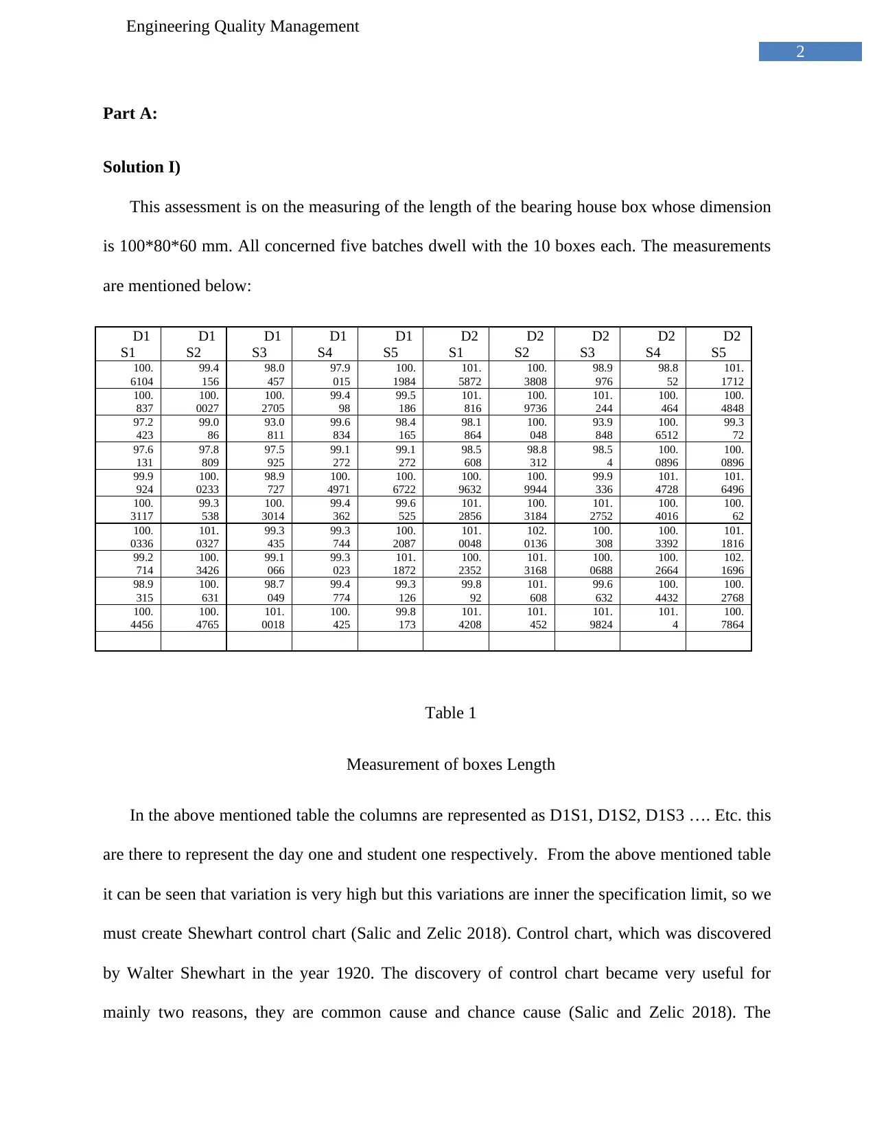
This assessment is on the measuring of the length of the bearing house box whose dimension
is 100*80*60 mm. All concerned five batches dwell with the 10 boxes each. The measurements
are mentioned below:
D1
S1
D1
S2
D1
S3
D1
S4
D1
S5
D2
S1
D2
S2
D2
S3
D2
S4
D2
S5
100.
6104
99.4
156
98.0
457
97.9
015
100.
1984
101.
5872
100.
3808
98.9
976
98.8
52
101.
1712
100.
837
100.
0027
100.
2705
99.4
98
99.5
186
101.
816
100.
9736
101.
244
100.
464
100.
4848
97.2
423
99.0
86
93.0
811
99.6
834
98.4
165
98.1
864
100.
048
93.9
848
100.
6512
99.3
72
97.6
131
97.8
809
97.5
925
99.1
272
99.1
272
98.5
608
98.8
312
98.5
4
100.
0896
100.
0896
99.9
924
100.
0233
98.9
727
100.
4971
100.
6722
100.
9632
100.
9944
99.9
336
101.
4728
101.
6496
100.
3117
99.3
538
100.
3014
99.4
362
99.6
525
101.
2856
100.
3184
101.
2752
100.
4016
100.
62
100.
0336
101.
0327
99.3
435
99.3
744
100.
2087
101.
0048
102.
0136
100.
308
100.
3392
101.
1816
99.2
714
100.
3426
99.1
066
99.3
023
101.
1872
100.
2352
101.
3168
100.
0688
100.
2664
102.
1696
98.9
315
100.
631
98.7
049
99.4
774
99.3
126
99.8
92
101.
608
99.6
632
100.
4432
100.
2768
100.
4456
100.
4765
101.
0018
100.
425
99.8
173
101.
4208
101.
452
101.
9824
101.
4
100.
7864
Table 1
Measurement of boxes Length
In the above mentioned table the columns are represented as D1S1, D1S2, D1S3 …. Etc. this
are there to represent the day one and student one respectively. From the above mentioned table
it can be seen that variation is very high but this variations are inner the specification limit, so we
must create Shewhart control chart (Salic and Zelic 2018). Control chart, which was discovered
by Walter Shewhart in the year 1920. The discovery of control chart became very useful for
mainly two reasons, they are common cause and chance cause (Salic and Zelic 2018). The
Engineering Quality Management
Part A:
Solution I)
This assessment is on the measuring of the length of the bearing house box whose dimension
is 100*80*60 mm. All concerned five batches dwell with the 10 boxes each. The measurements
are mentioned below:
D1
S1
D1
S2
D1
S3
D1
S4
D1
S5
D2
S1
D2
S2
D2
S3
D2
S4
D2
S5
100.
6104
99.4
156
98.0
457
97.9
015
100.
1984
101.
5872
100.
3808
98.9
976
98.8
52
101.
1712
100.
837
100.
0027
100.
2705
99.4
98
99.5
186
101.
816
100.
9736
101.
244
100.
464
100.
4848
97.2
423
99.0
86
93.0
811
99.6
834
98.4
165
98.1
864
100.
048
93.9
848
100.
6512
99.3
72
97.6
131
97.8
809
97.5
925
99.1
272
99.1
272
98.5
608
98.8
312
98.5
4
100.
0896
100.
0896
99.9
924
100.
0233
98.9
727
100.
4971
100.
6722
100.
9632
100.
9944
99.9
336
101.
4728
101.
6496
100.
3117
99.3
538
100.
3014
99.4
362
99.6
525
101.
2856
100.
3184
101.
2752
100.
4016
100.
62
100.
0336
101.
0327
99.3
435
99.3
744
100.
2087
101.
0048
102.
0136
100.
308
100.
3392
101.
1816
99.2
714
100.
3426
99.1
066
99.3
023
101.
1872
100.
2352
101.
3168
100.
0688
100.
2664
102.
1696
98.9
315
100.
631
98.7
049
99.4
774
99.3
126
99.8
92
101.
608
99.6
632
100.
4432
100.
2768
100.
4456
100.
4765
101.
0018
100.
425
99.8
173
101.
4208
101.
452
101.
9824
101.
4
100.
7864
Table 1
Measurement of boxes Length
In the above mentioned table the columns are represented as D1S1, D1S2, D1S3 …. Etc. this
are there to represent the day one and student one respectively. From the above mentioned table
it can be seen that variation is very high but this variations are inner the specification limit, so we
must create Shewhart control chart (Salic and Zelic 2018). Control chart, which was discovered
by Walter Shewhart in the year 1920. The discovery of control chart became very useful for
mainly two reasons, they are common cause and chance cause (Salic and Zelic 2018). The
⊘ This is a preview!⊘
Do you want full access?
Subscribe today to unlock all pages.
Trusted by 1+ million students worldwide
3
Engineering Quality Management
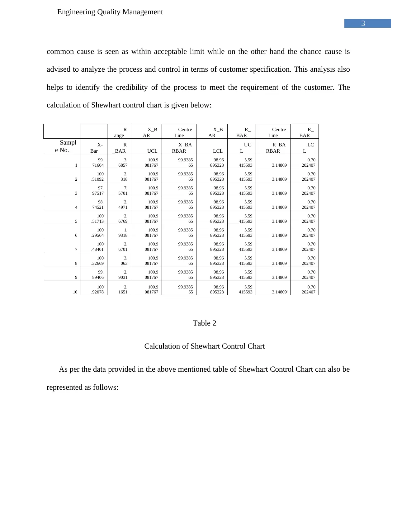
common cause is seen as within acceptable limit while on the other hand the chance cause is
advised to analyze the process and control in terms of customer specification. This analysis also
helps to identify the credibility of the process to meet the requirement of the customer. The
calculation of Shewhart control chart is given below:
R
ange
X_B
AR
Centre
Line
X_B
AR
R_
BAR
Centre
Line
R_
BAR
Sampl
e No. X-
Bar
R
_BAR UCL
X_BA
RBAR LCL
UC
L
R_BA
RBAR
LC
L
1
99.
71604
3.
6857
100.9
081767
99.9385
65
98.96
895328
5.59
415593 3.14809
0.70
202407
2
100
.51092
2.
318
100.9
081767
99.9385
65
98.96
895328
5.59
415593 3.14809
0.70
202407
3
97.
97517
7.
5701
100.9
081767
99.9385
65
98.96
895328
5.59
415593 3.14809
0.70
202407
4
98.
74521
2.
4971
100.9
081767
99.9385
65
98.96
895328
5.59
415593 3.14809
0.70
202407
5
100
.51713
2.
6769
100.9
081767
99.9385
65
98.96
895328
5.59
415593 3.14809
0.70
202407
6
100
.29564
1.
9318
100.9
081767
99.9385
65
98.96
895328
5.59
415593 3.14809
0.70
202407
7
100
.48401
2.
6701
100.9
081767
99.9385
65
98.96
895328
5.59
415593 3.14809
0.70
202407
8
100
.32669
3.
063
100.9
081767
99.9385
65
98.96
895328
5.59
415593 3.14809
0.70
202407
9
99.
89406
2.
9031
100.9
081767
99.9385
65
98.96
895328
5.59
415593 3.14809
0.70
202407
10
100
.92078
2.
1651
100.9
081767
99.9385
65
98.96
895328
5.59
415593 3.14809
0.70
202407
Table 2
Calculation of Shewhart Control Chart
As per the data provided in the above mentioned table of Shewhart Control Chart can also be
represented as follows:
Engineering Quality Management
common cause is seen as within acceptable limit while on the other hand the chance cause is
advised to analyze the process and control in terms of customer specification. This analysis also
helps to identify the credibility of the process to meet the requirement of the customer. The
calculation of Shewhart control chart is given below:
R
ange
X_B
AR
Centre
Line
X_B
AR
R_
BAR
Centre
Line
R_
BAR
Sampl
e No. X-
Bar
R
_BAR UCL
X_BA
RBAR LCL
UC
L
R_BA
RBAR
LC
L
1
99.
71604
3.
6857
100.9
081767
99.9385
65
98.96
895328
5.59
415593 3.14809
0.70
202407
2
100
.51092
2.
318
100.9
081767
99.9385
65
98.96
895328
5.59
415593 3.14809
0.70
202407
3
97.
97517
7.
5701
100.9
081767
99.9385
65
98.96
895328
5.59
415593 3.14809
0.70
202407
4
98.
74521
2.
4971
100.9
081767
99.9385
65
98.96
895328
5.59
415593 3.14809
0.70
202407
5
100
.51713
2.
6769
100.9
081767
99.9385
65
98.96
895328
5.59
415593 3.14809
0.70
202407
6
100
.29564
1.
9318
100.9
081767
99.9385
65
98.96
895328
5.59
415593 3.14809
0.70
202407
7
100
.48401
2.
6701
100.9
081767
99.9385
65
98.96
895328
5.59
415593 3.14809
0.70
202407
8
100
.32669
3.
063
100.9
081767
99.9385
65
98.96
895328
5.59
415593 3.14809
0.70
202407
9
99.
89406
2.
9031
100.9
081767
99.9385
65
98.96
895328
5.59
415593 3.14809
0.70
202407
10
100
.92078
2.
1651
100.9
081767
99.9385
65
98.96
895328
5.59
415593 3.14809
0.70
202407
Table 2
Calculation of Shewhart Control Chart
As per the data provided in the above mentioned table of Shewhart Control Chart can also be
represented as follows:
Paraphrase This Document
Need a fresh take? Get an instant paraphrase of this document with our AI Paraphraser
4
Engineering Quality Management
0 2 4 6 8 10 12
0
1
2
3
4
5
6
7
8
R_Bar Chart
R_BAR UCL Center Line LCL
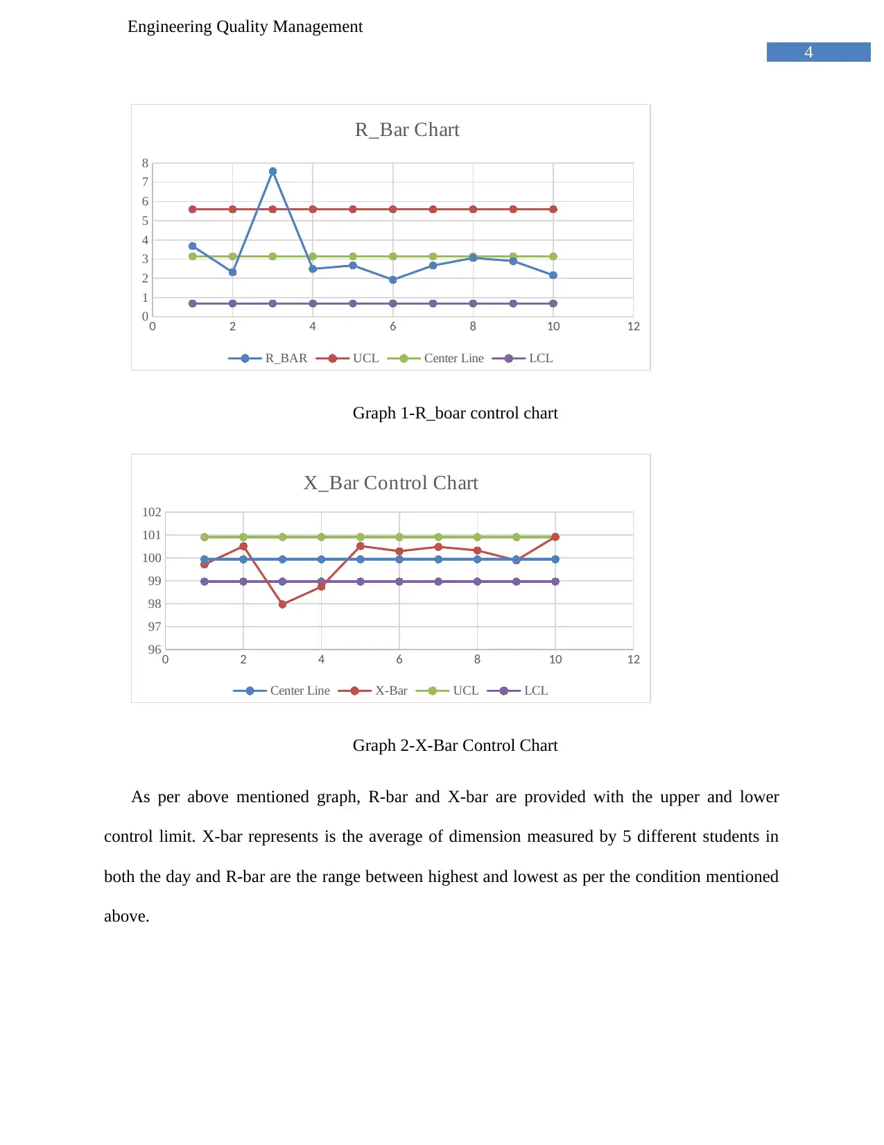
Graph 1-R_boar control chart
0 2 4 6 8 10 12
96
97
98
99
100
101
102
X_Bar Control Chart
Center Line X-Bar UCL LCL
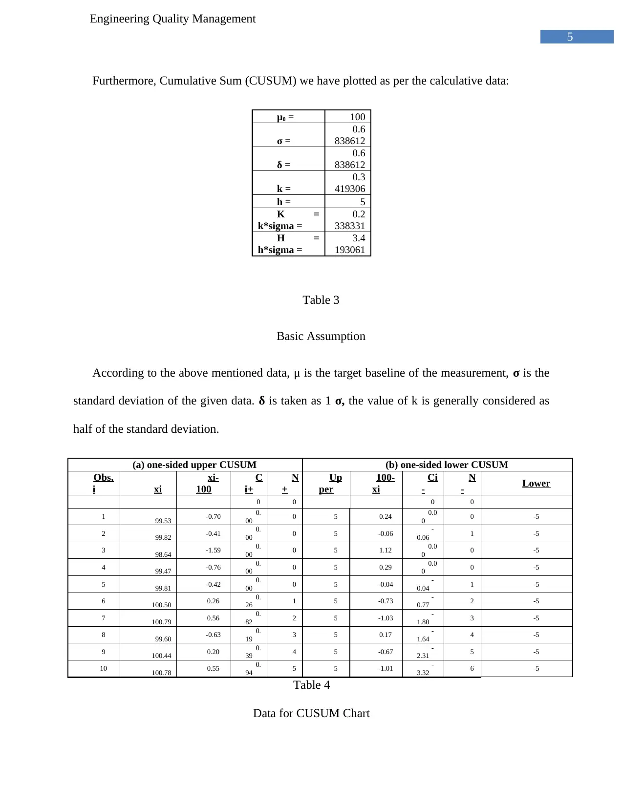
Graph 2-X-Bar Control Chart
As per above mentioned graph, R-bar and X-bar are provided with the upper and lower
control limit. X-bar represents is the average of dimension measured by 5 different students in
both the day and R-bar are the range between highest and lowest as per the condition mentioned
above.
Engineering Quality Management
0 2 4 6 8 10 12
0
1
2
3
4
5
6
7
8
R_Bar Chart
R_BAR UCL Center Line LCL
Graph 1-R_boar control chart
0 2 4 6 8 10 12
96
97
98
99
100
101
102
X_Bar Control Chart
Center Line X-Bar UCL LCL
Graph 2-X-Bar Control Chart
As per above mentioned graph, R-bar and X-bar are provided with the upper and lower
control limit. X-bar represents is the average of dimension measured by 5 different students in
both the day and R-bar are the range between highest and lowest as per the condition mentioned
above.
5
Engineering Quality Management
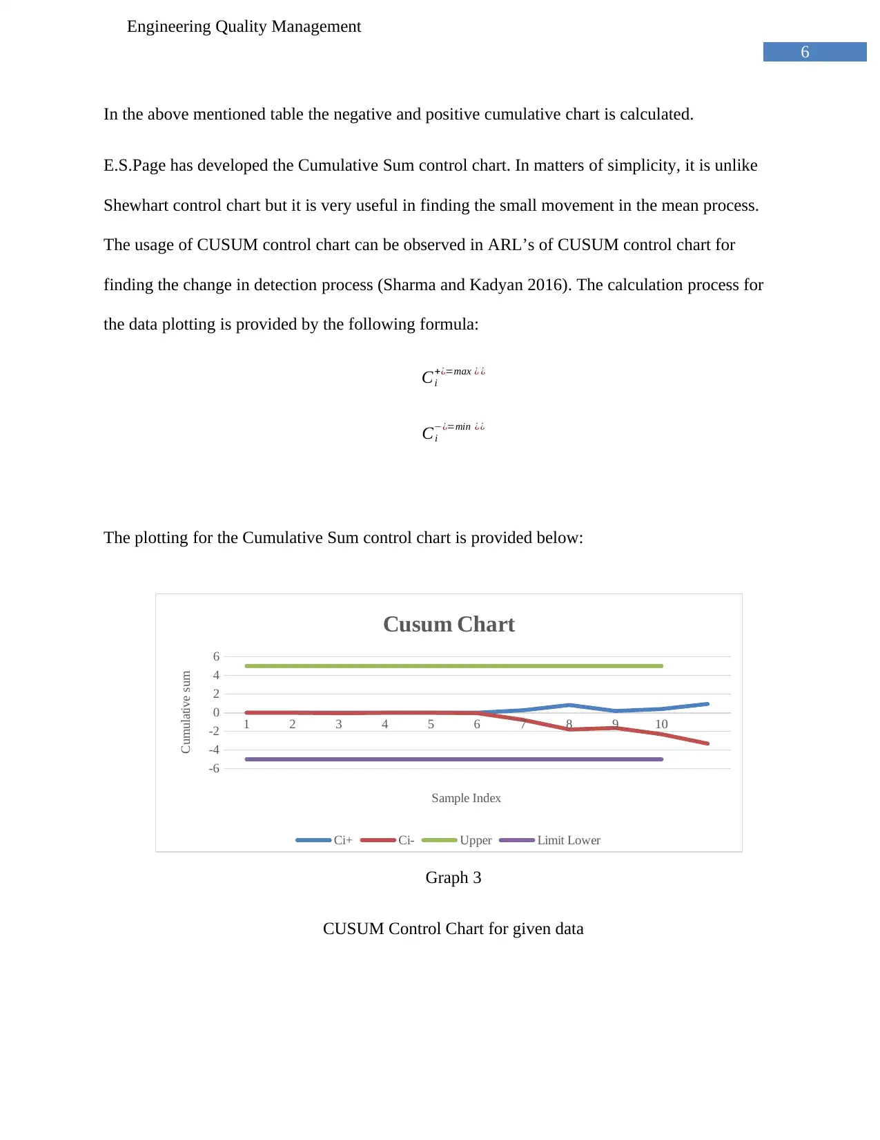
Furthermore, Cumulative Sum (CUSUM) we have plotted as per the calculative data:
μ0 = 100
σ =
0.6
838612
δ =
0.6
838612
k =
0.3
419306
h = 5
K =
k*sigma =
0.2
338331
H =
h*sigma =
3.4
193061
Table 3
Basic Assumption
According to the above mentioned data, μ is the target baseline of the measurement, σ is the
standard deviation of the given data. δ is taken as 1 σ, the value of k is generally considered as
half of the standard deviation.
(a) one-sided upper CUSUM (b) one-sided lower CUSUM
Obs,
i xi
xi-
100
C
i+
N
+
Up
per
100-
xi
Ci
-
N
- Lower
0 0 0 0
1 99.53 -0.70 0.
00 0 5 0.24 0.0
0 0 -5
2 99.82 -0.41 0.
00 0 5 -0.06 -
0.06 1 -5
3 98.64 -1.59 0.
00 0 5 1.12 0.0
0 0 -5
4 99.47 -0.76 0.
00 0 5 0.29 0.0
0 0 -5
5 99.81 -0.42 0.
00 0 5 -0.04 -
0.04 1 -5
6 100.50 0.26 0.
26 1 5 -0.73 -
0.77 2 -5
7 100.79 0.56 0.
82 2 5 -1.03 -
1.80 3 -5
8 99.60 -0.63 0.
19 3 5 0.17 -
1.64 4 -5
9 100.44 0.20 0.
39 4 5 -0.67 -
2.31 5 -5
10 100.78 0.55 0.
94 5 5 -1.01 -
3.32 6 -5
Table 4
Data for CUSUM Chart
Engineering Quality Management
Furthermore, Cumulative Sum (CUSUM) we have plotted as per the calculative data:
μ0 = 100
σ =
0.6
838612
δ =
0.6
838612
k =
0.3
419306
h = 5
K =
k*sigma =
0.2
338331
H =
h*sigma =
3.4
193061
Table 3
Basic Assumption
According to the above mentioned data, μ is the target baseline of the measurement, σ is the
standard deviation of the given data. δ is taken as 1 σ, the value of k is generally considered as
half of the standard deviation.
(a) one-sided upper CUSUM (b) one-sided lower CUSUM
Obs,
i xi
xi-
100
C
i+
N
+
Up
per
100-
xi
Ci
-
N
- Lower
0 0 0 0
1 99.53 -0.70 0.
00 0 5 0.24 0.0
0 0 -5
2 99.82 -0.41 0.
00 0 5 -0.06 -
0.06 1 -5
3 98.64 -1.59 0.
00 0 5 1.12 0.0
0 0 -5
4 99.47 -0.76 0.
00 0 5 0.29 0.0
0 0 -5
5 99.81 -0.42 0.
00 0 5 -0.04 -
0.04 1 -5
6 100.50 0.26 0.
26 1 5 -0.73 -
0.77 2 -5
7 100.79 0.56 0.
82 2 5 -1.03 -
1.80 3 -5
8 99.60 -0.63 0.
19 3 5 0.17 -
1.64 4 -5
9 100.44 0.20 0.
39 4 5 -0.67 -
2.31 5 -5
10 100.78 0.55 0.
94 5 5 -1.01 -
3.32 6 -5
Table 4
Data for CUSUM Chart
⊘ This is a preview!⊘
Do you want full access?
Subscribe today to unlock all pages.
Trusted by 1+ million students worldwide
6
Engineering Quality Management
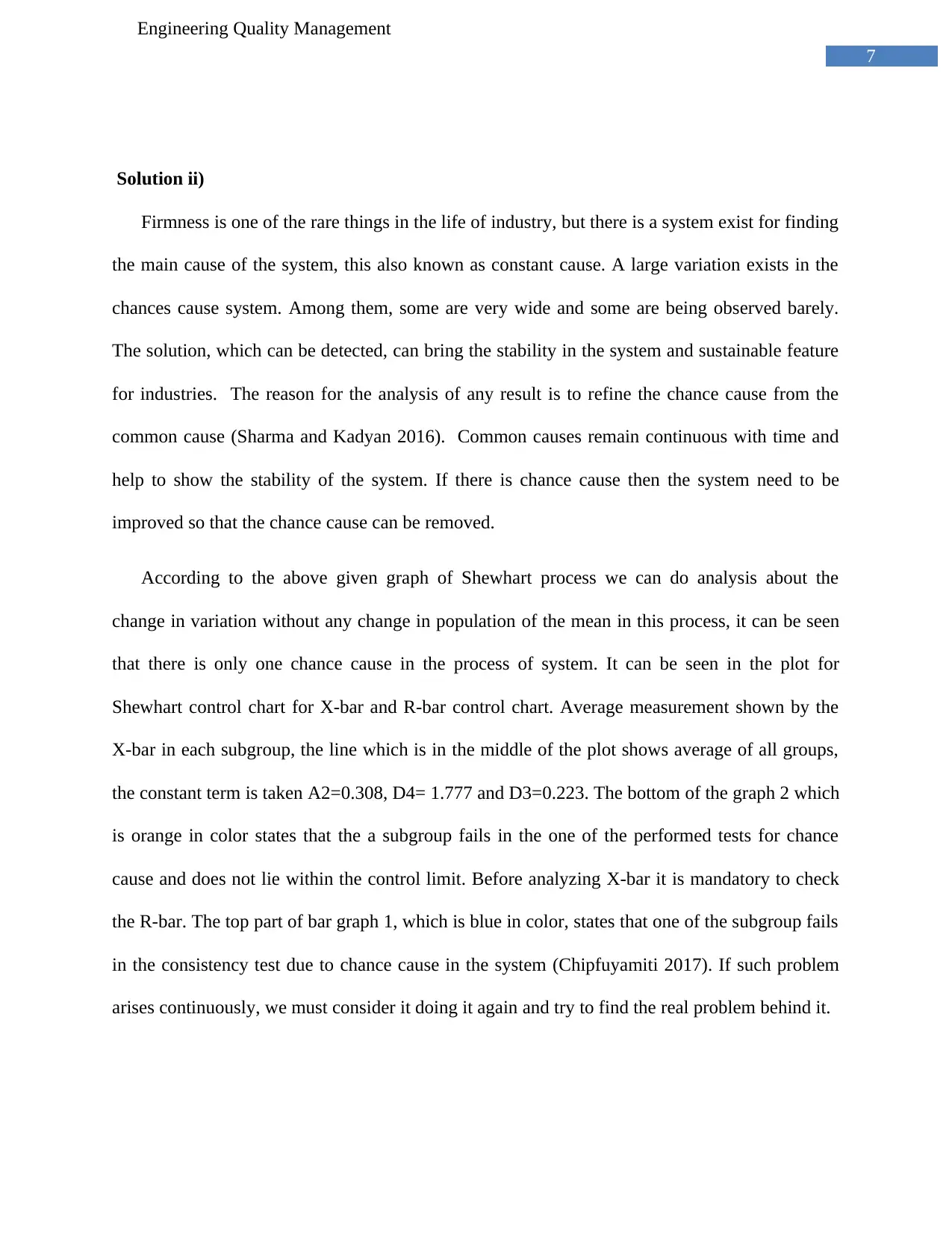
In the above mentioned table the negative and positive cumulative chart is calculated.
E.S.Page has developed the Cumulative Sum control chart. In matters of simplicity, it is unlike
Shewhart control chart but it is very useful in finding the small movement in the mean process.
The usage of CUSUM control chart can be observed in ARL’s of CUSUM control chart for
finding the change in detection process (Sharma and Kadyan 2016). The calculation process for
the data plotting is provided by the following formula:
Ci
+¿=max ¿ ¿
Ci
−¿=min ¿¿
The plotting for the Cumulative Sum control chart is provided below:
1 2 3 4 5 6 7 8 9 10
-6
-4
-2
0
2
4
6
Cusum Chart
Ci+ Ci- Upper Limit Lower
Sample Index
Cumulative sum
Graph 3
CUSUM Control Chart for given data
Engineering Quality Management
In the above mentioned table the negative and positive cumulative chart is calculated.
E.S.Page has developed the Cumulative Sum control chart. In matters of simplicity, it is unlike
Shewhart control chart but it is very useful in finding the small movement in the mean process.
The usage of CUSUM control chart can be observed in ARL’s of CUSUM control chart for
finding the change in detection process (Sharma and Kadyan 2016). The calculation process for
the data plotting is provided by the following formula:
Ci
+¿=max ¿ ¿
Ci
−¿=min ¿¿
The plotting for the Cumulative Sum control chart is provided below:
1 2 3 4 5 6 7 8 9 10
-6
-4
-2
0
2
4
6
Cusum Chart
Ci+ Ci- Upper Limit Lower
Sample Index
Cumulative sum
Graph 3
CUSUM Control Chart for given data
Paraphrase This Document
Need a fresh take? Get an instant paraphrase of this document with our AI Paraphraser
7
Engineering Quality Management
Solution ii)
Firmness is one of the rare things in the life of industry, but there is a system exist for finding
the main cause of the system, this also known as constant cause. A large variation exists in the
chances cause system. Among them, some are very wide and some are being observed barely.
The solution, which can be detected, can bring the stability in the system and sustainable feature
for industries. The reason for the analysis of any result is to refine the chance cause from the
common cause (Sharma and Kadyan 2016). Common causes remain continuous with time and
help to show the stability of the system. If there is chance cause then the system need to be
improved so that the chance cause can be removed.
According to the above given graph of Shewhart process we can do analysis about the
change in variation without any change in population of the mean in this process, it can be seen
that there is only one chance cause in the process of system. It can be seen in the plot for
Shewhart control chart for X-bar and R-bar control chart. Average measurement shown by the
X-bar in each subgroup, the line which is in the middle of the plot shows average of all groups,
the constant term is taken A2=0.308, D4= 1.777 and D3=0.223. The bottom of the graph 2 which
is orange in color states that the a subgroup fails in the one of the performed tests for chance
cause and does not lie within the control limit. Before analyzing X-bar it is mandatory to check
the R-bar. The top part of bar graph 1, which is blue in color, states that one of the subgroup fails
in the consistency test due to chance cause in the system (Chipfuyamiti 2017). If such problem
arises continuously, we must consider it doing it again and try to find the real problem behind it.
8
Engineering Quality Management
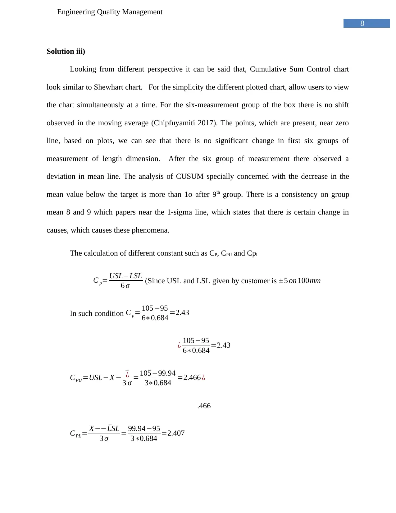
Solution iii)
Looking from different perspective it can be said that, Cumulative Sum Control chart
look similar to Shewhart chart. For the simplicity the different plotted chart, allow users to view
the chart simultaneously at a time. For the six-measurement group of the box there is no shift
observed in the moving average (Chipfuyamiti 2017). The points, which are present, near zero
line, based on plots, we can see that there is no significant change in first six groups of
measurement of length dimension. After the six group of measurement there observed a
deviation in mean line. The analysis of CUSUM specially concerned with the decrease in the
mean value below the target is more than 1σ after 9th group. There is a consistency on group
mean 8 and 9 which papers near the 1-sigma line, which states that there is certain change in
causes, which causes these phenomena.
The calculation of different constant such as CP, CPU and Cpl
C p= USL−LSL
6 σ (Since USL and LSL given by customer is ± 5 on 100mm
In such condition C p= 105−95
6∗0.684 =2.43
¿ 105−95
6∗0.684 =2.43
CPU =USL−X − ¯¿
3 σ =105−99.94
3∗0.684 =2.466 ¿
.466
CPL= X− ¯−LSL
3 σ = 99.94−95
3∗0.684 =2.407
Engineering Quality Management
Solution iii)
Looking from different perspective it can be said that, Cumulative Sum Control chart
look similar to Shewhart chart. For the simplicity the different plotted chart, allow users to view
the chart simultaneously at a time. For the six-measurement group of the box there is no shift
observed in the moving average (Chipfuyamiti 2017). The points, which are present, near zero
line, based on plots, we can see that there is no significant change in first six groups of
measurement of length dimension. After the six group of measurement there observed a
deviation in mean line. The analysis of CUSUM specially concerned with the decrease in the
mean value below the target is more than 1σ after 9th group. There is a consistency on group
mean 8 and 9 which papers near the 1-sigma line, which states that there is certain change in
causes, which causes these phenomena.
The calculation of different constant such as CP, CPU and Cpl
C p= USL−LSL
6 σ (Since USL and LSL given by customer is ± 5 on 100mm
In such condition C p= 105−95
6∗0.684 =2.43
¿ 105−95
6∗0.684 =2.43
CPU =USL−X − ¯¿
3 σ =105−99.94
3∗0.684 =2.466 ¿
.466
CPL= X− ¯−LSL
3 σ = 99.94−95
3∗0.684 =2.407
⊘ This is a preview!⊘
Do you want full access?
Subscribe today to unlock all pages.
Trusted by 1+ million students worldwide
9
Engineering Quality Management
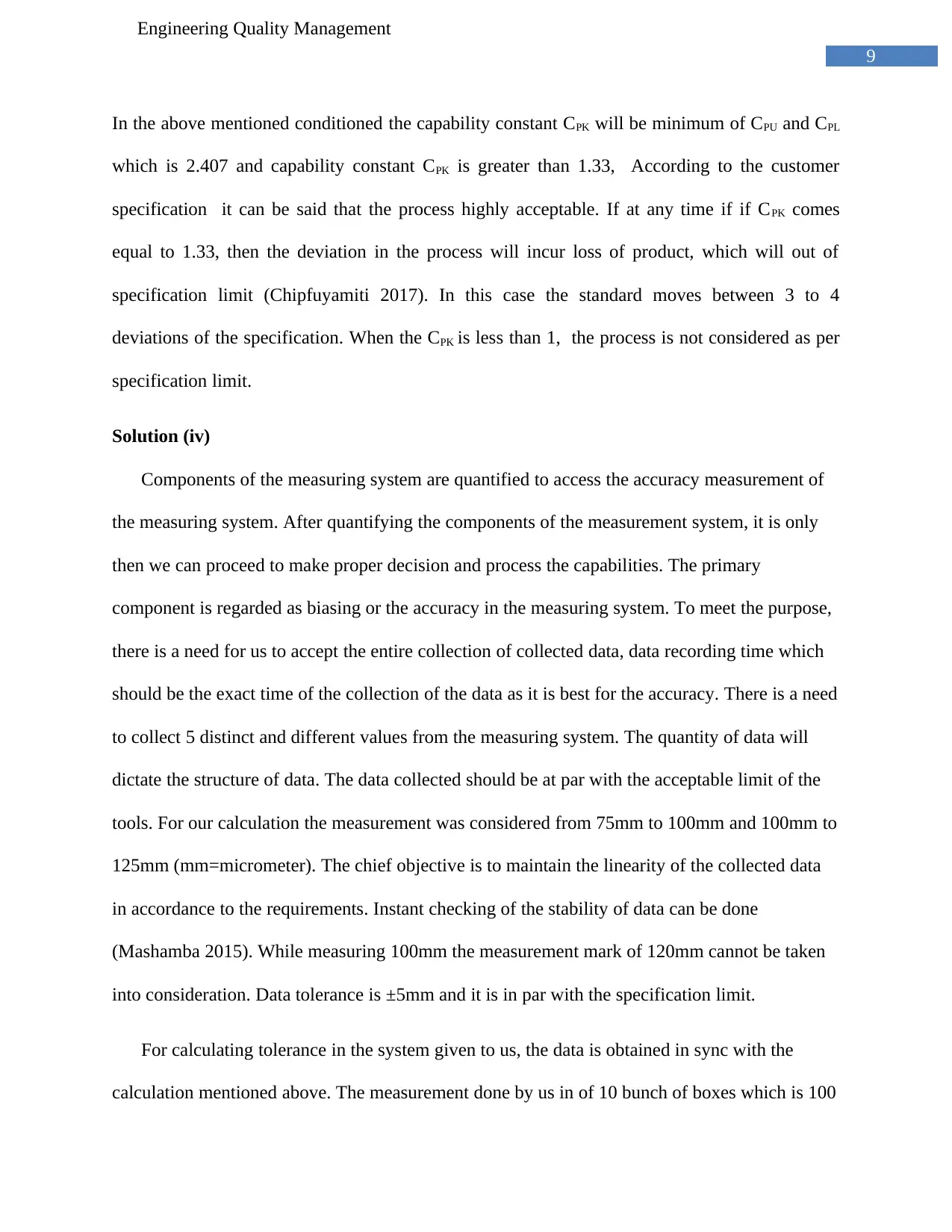
In the above mentioned conditioned the capability constant CPK will be minimum of CPU and CPL
which is 2.407 and capability constant CPK is greater than 1.33, According to the customer
specification it can be said that the process highly acceptable. If at any time if if CPK comes
equal to 1.33, then the deviation in the process will incur loss of product, which will out of
specification limit (Chipfuyamiti 2017). In this case the standard moves between 3 to 4
deviations of the specification. When the CPK is less than 1, the process is not considered as per
specification limit.
Solution (iv)
Components of the measuring system are quantified to access the accuracy measurement of
the measuring system. After quantifying the components of the measurement system, it is only
then we can proceed to make proper decision and process the capabilities. The primary
component is regarded as biasing or the accuracy in the measuring system. To meet the purpose,
there is a need for us to accept the entire collection of collected data, data recording time which
should be the exact time of the collection of the data as it is best for the accuracy. There is a need
to collect 5 distinct and different values from the measuring system. The quantity of data will
dictate the structure of data. The data collected should be at par with the acceptable limit of the
tools. For our calculation the measurement was considered from 75mm to 100mm and 100mm to
125mm (mm=micrometer). The chief objective is to maintain the linearity of the collected data
in accordance to the requirements. Instant checking of the stability of data can be done
(Mashamba 2015). While measuring 100mm the measurement mark of 120mm cannot be taken
into consideration. Data tolerance is ±5mm and it is in par with the specification limit.
For calculating tolerance in the system given to us, the data is obtained in sync with the
calculation mentioned above. The measurement done by us in of 10 bunch of boxes which is 100
Engineering Quality Management
In the above mentioned conditioned the capability constant CPK will be minimum of CPU and CPL
which is 2.407 and capability constant CPK is greater than 1.33, According to the customer
specification it can be said that the process highly acceptable. If at any time if if CPK comes
equal to 1.33, then the deviation in the process will incur loss of product, which will out of
specification limit (Chipfuyamiti 2017). In this case the standard moves between 3 to 4
deviations of the specification. When the CPK is less than 1, the process is not considered as per
specification limit.
Solution (iv)
Components of the measuring system are quantified to access the accuracy measurement of
the measuring system. After quantifying the components of the measurement system, it is only
then we can proceed to make proper decision and process the capabilities. The primary
component is regarded as biasing or the accuracy in the measuring system. To meet the purpose,
there is a need for us to accept the entire collection of collected data, data recording time which
should be the exact time of the collection of the data as it is best for the accuracy. There is a need
to collect 5 distinct and different values from the measuring system. The quantity of data will
dictate the structure of data. The data collected should be at par with the acceptable limit of the
tools. For our calculation the measurement was considered from 75mm to 100mm and 100mm to
125mm (mm=micrometer). The chief objective is to maintain the linearity of the collected data
in accordance to the requirements. Instant checking of the stability of data can be done
(Mashamba 2015). While measuring 100mm the measurement mark of 120mm cannot be taken
into consideration. Data tolerance is ±5mm and it is in par with the specification limit.
For calculating tolerance in the system given to us, the data is obtained in sync with the
calculation mentioned above. The measurement done by us in of 10 bunch of boxes which is 100
Paraphrase This Document
Need a fresh take? Get an instant paraphrase of this document with our AI Paraphraser
10
Engineering Quality Management
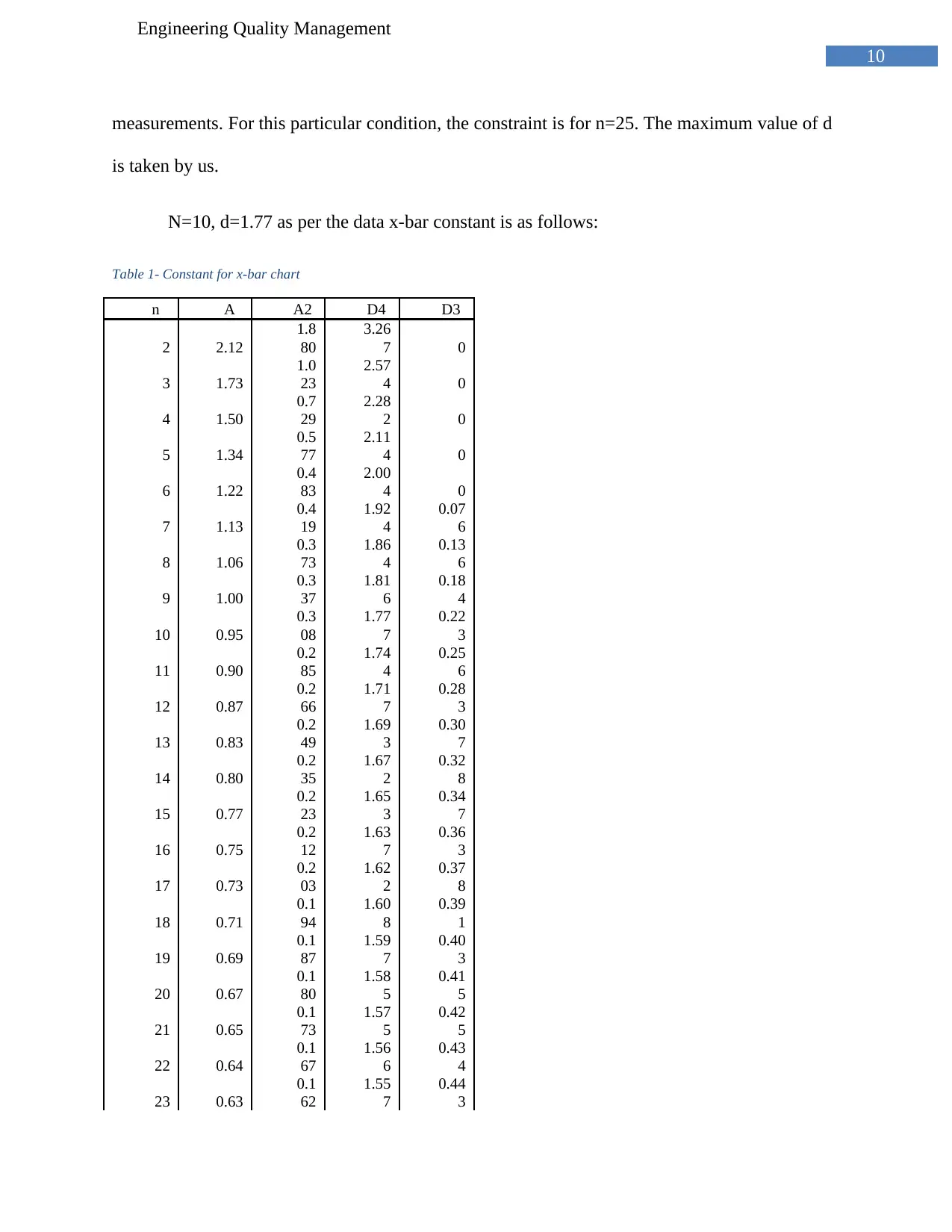
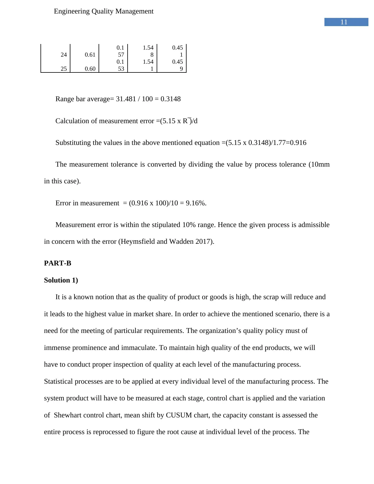
measurements. For this particular condition, the constraint is for n=25. The maximum value of d
is taken by us.
N=10, d=1.77 as per the data x-bar constant is as follows:
Table 1- Constant for x-bar chart
n A A2 D4 D3
2 2.12
1.8
80
3.26
7 0
3 1.73
1.0
23
2.57
4 0
4 1.50
0.7
29
2.28
2 0
5 1.34
0.5
77
2.11
4 0
6 1.22
0.4
83
2.00
4 0
7 1.13
0.4
19
1.92
4
0.07
6
8 1.06
0.3
73
1.86
4
0.13
6
9 1.00
0.3
37
1.81
6
0.18
4
10 0.95
0.3
08
1.77
7
0.22
3
11 0.90
0.2
85
1.74
4
0.25
6
12 0.87
0.2
66
1.71
7
0.28
3
13 0.83
0.2
49
1.69
3
0.30
7
14 0.80
0.2
35
1.67
2
0.32
8
15 0.77
0.2
23
1.65
3
0.34
7
16 0.75
0.2
12
1.63
7
0.36
3
17 0.73
0.2
03
1.62
2
0.37
8
18 0.71
0.1
94
1.60
8
0.39
1
19 0.69
0.1
87
1.59
7
0.40
3
20 0.67
0.1
80
1.58
5
0.41
5
21 0.65
0.1
73
1.57
5
0.42
5
22 0.64
0.1
67
1.56
6
0.43
4
23 0.63
0.1
62
1.55
7
0.44
3
Engineering Quality Management
measurements. For this particular condition, the constraint is for n=25. The maximum value of d
is taken by us.
N=10, d=1.77 as per the data x-bar constant is as follows:
Table 1- Constant for x-bar chart
n A A2 D4 D3
2 2.12
1.8
80
3.26
7 0
3 1.73
1.0
23
2.57
4 0
4 1.50
0.7
29
2.28
2 0
5 1.34
0.5
77
2.11
4 0
6 1.22
0.4
83
2.00
4 0
7 1.13
0.4
19
1.92
4
0.07
6
8 1.06
0.3
73
1.86
4
0.13
6
9 1.00
0.3
37
1.81
6
0.18
4
10 0.95
0.3
08
1.77
7
0.22
3
11 0.90
0.2
85
1.74
4
0.25
6
12 0.87
0.2
66
1.71
7
0.28
3
13 0.83
0.2
49
1.69
3
0.30
7
14 0.80
0.2
35
1.67
2
0.32
8
15 0.77
0.2
23
1.65
3
0.34
7
16 0.75
0.2
12
1.63
7
0.36
3
17 0.73
0.2
03
1.62
2
0.37
8
18 0.71
0.1
94
1.60
8
0.39
1
19 0.69
0.1
87
1.59
7
0.40
3
20 0.67
0.1
80
1.58
5
0.41
5
21 0.65
0.1
73
1.57
5
0.42
5
22 0.64
0.1
67
1.56
6
0.43
4
23 0.63
0.1
62
1.55
7
0.44
3
11
Engineering Quality Management
24 0.61
0.1
57
1.54
8
0.45
1
25 0.60
0.1
53
1.54
1
0.45
9
Range bar average= 31.481 / 100 = 0.3148
Calculation of measurement error =(5.15 x R ̅ )/d
Substituting the values in the above mentioned equation =(5.15 x 0.3148)/1.77=0.916
The measurement tolerance is converted by dividing the value by process tolerance (10mm
in this case).
Error in measurement = (0.916 x 100)/10 = 9.16%.
Measurement error is within the stipulated 10% range. Hence the given process is admissible
in concern with the error (Heymsfield and Wadden 2017).
PART-B
Solution 1)
It is a known notion that as the quality of product or goods is high, the scrap will reduce and
it leads to the highest value in market share. In order to achieve the mentioned scenario, there is a
need for the meeting of particular requirements. The organization’s quality policy must of
immense prominence and immaculate. To maintain high quality of the end products, we will
have to conduct proper inspection of quality at each level of the manufacturing process.
Statistical processes are to be applied at every individual level of the manufacturing process. The
system product will have to be measured at each stage, control chart is applied and the variation
of Shewhart control chart, mean shift by CUSUM chart, the capacity constant is assessed the
entire process is reprocessed to figure the root cause at individual level of the process. The
⊘ This is a preview!⊘
Do you want full access?
Subscribe today to unlock all pages.
Trusted by 1+ million students worldwide
1 out of 15
Your All-in-One AI-Powered Toolkit for Academic Success.
+13062052269
info@desklib.com
Available 24*7 on WhatsApp / Email
![[object Object]](/_next/static/media/star-bottom.7253800d.svg)
Unlock your academic potential
Copyright © 2020–2026 A2Z Services. All Rights Reserved. Developed and managed by ZUCOL.