ENG3104: Engineering Simulations and Computations Assignment 2

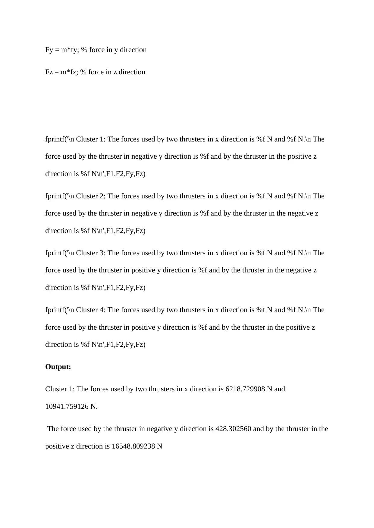
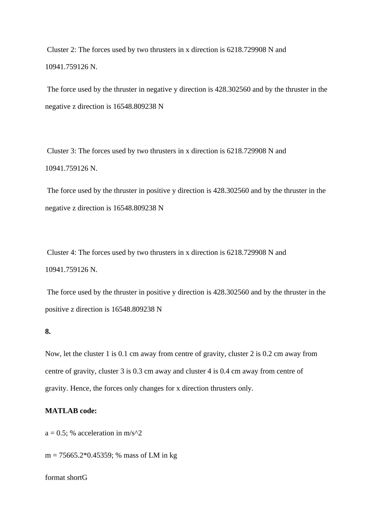
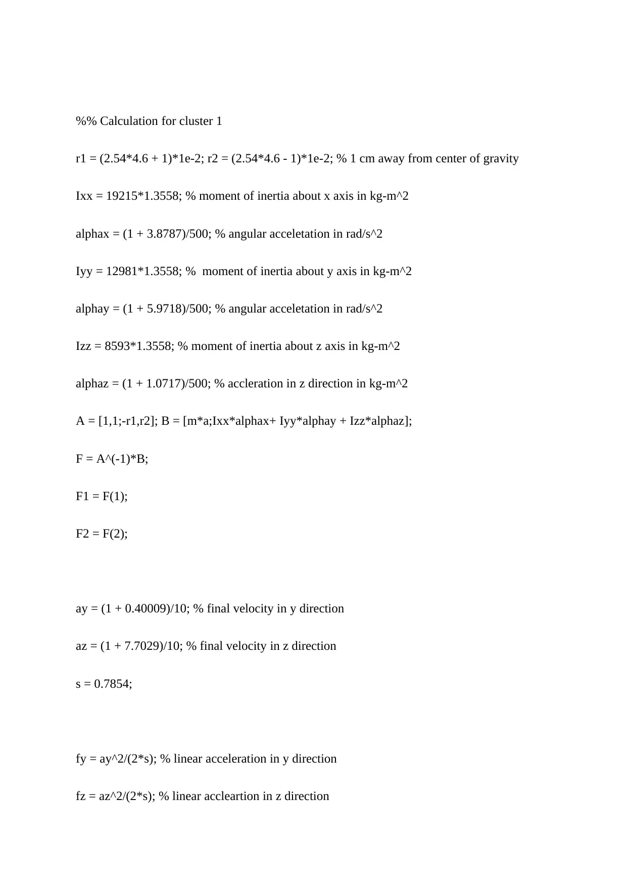
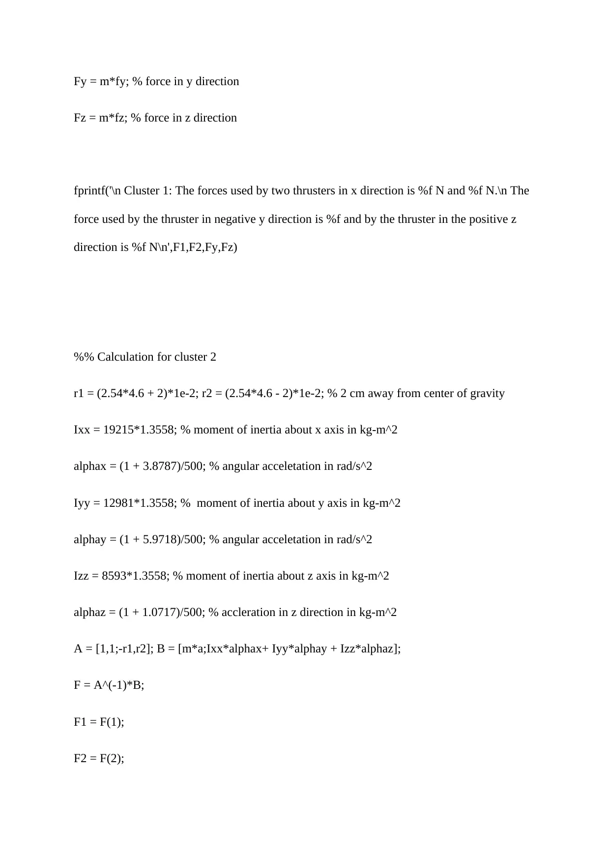
This assignment solution for ENG3104 focuses on simulating the landing of the Apollo 11 Lunar Module (LM). The solution begins by calculating the force required for a given linear acceleration using Newton's second law, considering the mass of the LM. It then analyzes the forces and moments involved when thrusters are not aligned with the center of gravity, using simultaneous equations and matrix methods to determine individual thruster forces. The solution incorporates MATLAB code to verify the calculations, including scenarios with angular acceleration and forces in multiple directions. The document then explores the impact of thrusters in the y and z directions, and how the location of thrusters affects the force distribution. The document presents the calculations for different cluster configurations, and how the forces change based on the distance from the center of gravity. The solution includes detailed MATLAB code and output for each scenario, providing a comprehensive understanding of the LM's control system during descent.

Running head: ASSIGNMENT 2
ASSIGNMENT 2
Name of the Student
Name of the University
Author Note

Question 1:
Lnar module acceleration = 0.5 m/s^2.
LM properties in empirical units:
Mass m of LM = 75665.2 lb = 75665.2*0.45359 = 34321.157 kgs.
Therefore, F = 34321.157*0.5 = 17160.5785 N.
Now, by balancing forces in x direction
F1+F2=ma (2)
F2∗r2 – F1∗r1=I xx∗αx (3)
Given I xx = 19215 slug.ft^2 = 19215*1.3558 kg-m^2 = 26052.04 kg-m^2.
Now, linear acceleration in the positive y-direction is 0.5 m/s^2 or a = 0.5 m/s^2.
Now, the angular acceleration in x-direction is 0.25°/s^2 or αx = 0.25°/s^2 = 0.004 rad/s^2
F1+F2=34321.157∗0.5 (A)
Now, from figure 4, the distance of applied forces F1 and F2 from x axis is equal to 4.6’’.
Hence, r1 = r2 = 4.6’’ = 0.116 m.
Hence, substituting in equation (3)
F2∗0.116 – F1∗0.116=26052.04∗0.004
 F2 – F1 = 898.346 (B)

Now, solving (A) and (B) gives
F1 = 8131.1 N.
F2 = 9029.5 N.
Now, (2) and (3) in matrix form is given by,
[ 1 1
−r 1 r 2 ][ F 1
F 2 ] =
[ ma
I xx∗αx ]
Putting values,
[ 1 1
−0.116 0.116 ][ F 1
F 2 ] = [ 34321.157∗0.5
26052.04∗0.004 ]
Hence, [ F 1
F 2 ] = [ 1 1
−0.116 0.116 ]−1
[ 34321.157∗0.5
26052.04∗0.004 ]
[ F 1
F 2 ] = [ 8131.1
9029.5 ]
The above results are verified by MATLAB as given below.
MATLAB code:
a = 0.5; % acceleration in m/s^2
m = 75665.2*0.45359; % mass of LM
format shortG
F = m*a
r1 = 0.116; r2 = r1; % the distance of applied forces F1 and F2 from x axis
Ixx = 19215*1.3558; % moment of inertia about x axis in kg-m^2

alphax = (0.25*pi)/180; % angular acceletation in rad/s^2
A = [1,1;-0.116,0.116]; B = [m*a;Ixx*alphax];
F = A^(-1)*B;
F1 = F(1)
F2 = F(2)
Output:
q1r4
F =
17160
F1 =
8090.3
F2 =
9070.2
5.
Now, given ay = [(1 + 0.40009) / 10] m/s and α x = (1 + 3.8787)/500 rad/s^2.
Now, angular displacement from Fig 4 in y direction is 45° = 0.7854 rad.
Now, acceleration in the y direction is found from the equation
v^2 = u^2 + 2*f*s (u = 0 as before applying force there was no velocity in y direction)
 f = v^2/(2*s)
Hence by the y direction will be by thruster is F = m*f

MATLAB code:
a = 0.5; % acceleration in m/s^2
m = 75665.2*0.45359; % mass of LM in kg
format shortG
F = m*a;
r1 = 0.116; r2 = r1; % the distance of applied forces F1 and F2 from x axis
Ixx = 19215*1.3558; % moment of inertia about x axis in kg-m^2
alphax = (1 + 3.8787)/500; % angular acceletation in rad/s^2
A = [1,1;-0.116,0.116]; B = [m*a;Ixx*alphax];
F = A^(-1)*B;
F1 = F(1);
F2 = F(2);
ay = (1 + 0.40009)/10; % final velocity in y direction
s = 0.7854;
fy = ay^2/(2*s);
Fy = m*fy;
fprintf('\n The forces used by two thrusters in x direction is %f N and %f N. The force used
by the thruster in y direction is %f N \n',F1,F2,Fy)

Output:
The forces used by two thrusters in x direction is 7484.568533 N and 9675.920501 N. The
force used by the thruster in negative y direction is 428.302560 N
6.
MATLAB code:
a = 0.5; % acceleration in m/s^2
m = 75665.2*0.45359; % mass of LM in kg
format shortG
F = m*a;
r1 = 0.116; r2 = r1; % the distance of applied forces F1 and F2 from x axis
Ixx = 19215*1.3558; % moment of inertia about x axis in kg-m^2
alphax = (1 + 3.8787)/500; % angular acceletation in rad/s^2
A = [1,1;-0.116,0.116]; B = [m*a;Ixx*alphax];
F = A^(-1)*B;
F1 = F(1);
F2 = F(2);
ay = (1 + 0.40009)/10; % final velocity in y direction
az = (1 + 7.7029)/10; % final velocity in z direction
s = 0.7854;

fy = ay^2/(2*s); % linear acceleration in y direction
fz = az^2/(2*s); % linear accleartion in z direction
Fy = m*fy; % force in y direction
Fz = m*fz; % force in z direction
fprintf('\n Cluster 2: The forces used by two thrusters in x direction is %f N and %f N.\n The
force used by the thruster in negative y direction is %f and by the thruster in the negative z
direction is %f N\n',F1,F2,Fy,Fz)
Output:
Cluster 2: The forces used by two thrusters in x direction is 7484.568533 N and 9675.920501
N.
The force used by the thruster in negative y direction is 428.302560 and by the thruster in the
negative z direction is 16548.809238 N
7.
Now, the velocities and acceleration in all the direction is considered. Hence, the matrix
equation becomes
[ 1 1
−r 1 r 2 ][ F 1
F 2 ] =
[ ma
Ixx∗α x+ I yy∗α y + Izz∗αz ]
Hence, [ F 1
F 2 ] = [ 1 1
−r 1 r 2 ]−1
[ ma
Ixx∗α x+I yy∗α y + I zz∗αz ]
MATLAB code:
a = 0.5; % acceleration in m/s^2

m = 75665.2*0.45359; % mass of LM in kg
format shortG
r1 = 0.116; r2 = r1; % the distance of applied forces F1 and F2 from x axis in meters
Ixx = 19215*1.3558; % moment of inertia about x axis in kg-m^2
alphax = (1 + 3.8787)/500; % angular acceletation in rad/s^2
Iyy = 12981*1.3558; % moment of inertia about y axis in kg-m^2
alphay = (1 + 5.9718)/500; % angular acceletation in rad/s^2
Izz = 8593*1.3558; % moment of inertia about z axis in kg-m^2
alphaz = (1 + 1.0717)/500; % accleration in z direction in kg-m^2
A = [1,1;-0.116,0.116]; B = [m*a;Ixx*alphax+ Iyy*alphay + Izz*alphaz];
F = A^(-1)*B;
F1 = F(1);
F2 = F(2);
ay = (1 + 0.40009)/10; % final velocity in y direction
az = (1 + 7.7029)/10; % final velocity in z direction
s = 0.7854;
fy = ay^2/(2*s); % linear acceleration in y direction
fz = az^2/(2*s); % linear accleartion in z direction

Fy = m*fy; % force in y direction
Fz = m*fz; % force in z direction
fprintf('\n Cluster 1: The forces used by two thrusters in x direction is %f N and %f N.\n The
force used by the thruster in negative y direction is %f and by the thruster in the positive z
direction is %f N\n',F1,F2,Fy,Fz)
fprintf('\n Cluster 2: The forces used by two thrusters in x direction is %f N and %f N.\n The
force used by the thruster in negative y direction is %f and by the thruster in the negative z
direction is %f N\n',F1,F2,Fy,Fz)
fprintf('\n Cluster 3: The forces used by two thrusters in x direction is %f N and %f N.\n The
force used by the thruster in positive y direction is %f and by the thruster in the negative z
direction is %f N\n',F1,F2,Fy,Fz)
fprintf('\n Cluster 4: The forces used by two thrusters in x direction is %f N and %f N.\n The
force used by the thruster in positive y direction is %f and by the thruster in the positive z
direction is %f N\n',F1,F2,Fy,Fz)
Output:
Cluster 1: The forces used by two thrusters in x direction is 6218.729908 N and
10941.759126 N.
The force used by the thruster in negative y direction is 428.302560 and by the thruster in the
positive z direction is 16548.809238 N

Cluster 2: The forces used by two thrusters in x direction is 6218.729908 N and
10941.759126 N.
The force used by the thruster in negative y direction is 428.302560 and by the thruster in the
negative z direction is 16548.809238 N
Cluster 3: The forces used by two thrusters in x direction is 6218.729908 N and
10941.759126 N.
The force used by the thruster in positive y direction is 428.302560 and by the thruster in the
negative z direction is 16548.809238 N
Cluster 4: The forces used by two thrusters in x direction is 6218.729908 N and
10941.759126 N.
The force used by the thruster in positive y direction is 428.302560 and by the thruster in the
positive z direction is 16548.809238 N
8.
Now, let the cluster 1 is 0.1 cm away from centre of gravity, cluster 2 is 0.2 cm away from
centre of gravity, cluster 3 is 0.3 cm away and cluster 4 is 0.4 cm away from centre of
gravity. Hence, the forces only changes for x direction thrusters only.
MATLAB code:
a = 0.5; % acceleration in m/s^2
m = 75665.2*0.45359; % mass of LM in kg
format shortG

%% Calculation for cluster 1
r1 = (2.54*4.6 + 1)*1e-2; r2 = (2.54*4.6 - 1)*1e-2; % 1 cm away from center of gravity
Ixx = 19215*1.3558; % moment of inertia about x axis in kg-m^2
alphax = (1 + 3.8787)/500; % angular acceletation in rad/s^2
Iyy = 12981*1.3558; % moment of inertia about y axis in kg-m^2
alphay = (1 + 5.9718)/500; % angular acceletation in rad/s^2
Izz = 8593*1.3558; % moment of inertia about z axis in kg-m^2
alphaz = (1 + 1.0717)/500; % accleration in z direction in kg-m^2
A = [1,1;-r1,r2]; B = [m*a;Ixx*alphax+ Iyy*alphay + Izz*alphaz];
F = A^(-1)*B;
F1 = F(1);
F2 = F(2);
ay = (1 + 0.40009)/10; % final velocity in y direction
az = (1 + 7.7029)/10; % final velocity in z direction
s = 0.7854;
fy = ay^2/(2*s); % linear acceleration in y direction
fz = az^2/(2*s); % linear accleartion in z direction

Fy = m*fy; % force in y direction
Fz = m*fz; % force in z direction
fprintf('\n Cluster 1: The forces used by two thrusters in x direction is %f N and %f N.\n The
force used by the thruster in negative y direction is %f and by the thruster in the positive z
direction is %f N\n',F1,F2,Fy,Fz)
%% Calculation for cluster 2
r1 = (2.54*4.6 + 2)*1e-2; r2 = (2.54*4.6 - 2)*1e-2; % 2 cm away from center of gravity
Ixx = 19215*1.3558; % moment of inertia about x axis in kg-m^2
alphax = (1 + 3.8787)/500; % angular acceletation in rad/s^2
Iyy = 12981*1.3558; % moment of inertia about y axis in kg-m^2
alphay = (1 + 5.9718)/500; % angular acceletation in rad/s^2
Izz = 8593*1.3558; % moment of inertia about z axis in kg-m^2
alphaz = (1 + 1.0717)/500; % accleration in z direction in kg-m^2
A = [1,1;-r1,r2]; B = [m*a;Ixx*alphax+ Iyy*alphay + Izz*alphaz];
F = A^(-1)*B;
F1 = F(1);
F2 = F(2);

ay = (1 + 0.40009)/10; % final velocity in y direction
az = (1 + 7.7029)/10; % final velocity in z direction
s = 0.7854;
fy = ay^2/(2*s); % linear acceleration in y direction
fz = az^2/(2*s); % linear accleartion in z direction
Fy = m*fy; % force in y direction
Fz = m*fz; % force in z direction
fprintf('\n Cluster 2: The forces used by two thrusters in x direction is %f N and %f N.\n The
force used by the thruster in negative y direction is %f and by the thruster in the negative z
direction is %f N\n',F1,F2,Fy,Fz)
%% Calculation for cluster 3
r1 = (2.54*4.6 + 3)*1e-2; r2 = (2.54*4.6 - 3)*1e-2; % 3 cm away from center of gravity
Ixx = 19215*1.3558; % moment of inertia about x axis in kg-m^2
alphax = (1 + 3.8787)/500; % angular acceletation in rad/s^2
Iyy = 12981*1.3558; % moment of inertia about y axis in kg-m^2
alphay = (1 + 5.9718)/500; % angular acceletation in rad/s^2
Izz = 8593*1.3558; % moment of inertia about z axis in kg-m^2

alphaz = (1 + 1.0717)/500; % accleration in z direction in kg-m^2
A = [1,1;-r1,r2]; B = [m*a;Ixx*alphax+ Iyy*alphay + Izz*alphaz];
F = A^(-1)*B;
F1 = F(1);
F2 = F(2);
ay = (1 + 0.40009)/10; % final velocity in y direction
az = (1 + 7.7029)/10; % final velocity in z direction
s = 0.7854;
fy = ay^2/(2*s); % linear acceleration in y direction
fz = az^2/(2*s); % linear accleartion in z direction
Fy = m*fy; % force in y direction
Fz = m*fz; % force in z direction
fprintf('\n Cluster 3: The forces used by two thrusters in x direction is %f N and %f N.\n The
force used by the thruster in positive y direction is %f and by the thruster in the negative z
direction is %f N\n',F1,F2,Fy,Fz)
%% Calculation for cluster 4

r1 = (2.54*4.6 + 4)*1e-2; r2 = (2.54*4.6 - 4)*1e-2; % 4 cm away from center of gravity
Ixx = 19215*1.3558; % moment of inertia about x axis in kg-m^2
alphax = (1 + 3.8787)/500; % angular acceletation in rad/s^2
Iyy = 12981*1.3558; % moment of inertia about y axis in kg-m^2
alphay = (1 + 5.9718)/500; % angular acceletation in rad/s^2
Izz = 8593*1.3558; % moment of inertia about z axis in kg-m^2
alphaz = (1 + 1.0717)/500; % accleration in z direction in kg-m^2
A = [1,1;-r1,r2]; B = [m*a;Ixx*alphax+ Iyy*alphay + Izz*alphaz];
F = A^(-1)*B;
F1 = F(1);
F2 = F(2);
ay = (1 + 0.40009)/10; % final velocity in y direction
az = (1 + 7.7029)/10; % final velocity in z direction
s = 0.7854;
fy = ay^2/(2*s); % linear acceleration in y direction
fz = az^2/(2*s); % linear accleartion in z direction
Fy = m*fy; % force in y direction
Fz = m*fz; % force in z direction

fprintf('\n Cluster 4: The forces used by two thrusters in x direction is %f N and %f N.\n The
force used by the thruster in positive y direction is %f and by the thruster in the positive z
direction is %f N\n',F1,F2,Fy,Fz)
Output:
Cluster 1: The forces used by two thrusters in x direction is 5501.349106 N and
11659.139928 N.
The force used by the thruster in negative y direction is 428.302560 and by the thruster in the
positive z direction is 16548.809238 N
Cluster 2: The forces used by two thrusters in x direction is 4766.990623 N and
12393.498411 N.
The force used by the thruster in negative y direction is 428.302560 and by the thruster in the
negative z direction is 16548.809238 N
Cluster 3: The forces used by two thrusters in x direction is 4032.632140 N and
13127.856894 N.
The force used by the thruster in positive y direction is 428.302560 and by the thruster in the
negative z direction is 16548.809238 N
Cluster 4: The forces used by two thrusters in x direction is 3298.273657 N and
13862.215377 N.

The force used by the thruster in positive y direction is 428.302560 and by the thruster in the
positive z direction is 16548.809238 N
Question 2:
The first two values of altitude when alarm 1201 was active are 2480 ft and 2290 ft
respectively. Also, at the same instants the range in ft are 9840 ft and 9150 ft respectively.
Now, by linear regression of curve fitting the range as a function of altitude will be.
Range = a + b*alt
a = ((∑ y ¿∗(∑ x2 )−(∑ x )(∑ xy )¿ /¿ = 833.68
b = (n( ∑ xy ¿−(∑ x )(∑ y )¿ /¿ = 3.6316
Now, by fitting logarithmic function to the data
Range = a + b*ln(alt)
The estimates of a and b will be
Range = -57821 + 8656.7*ln(alt)
Now, power series is fitted with the data.
Range=a∗ ( alt ) b
The estimates of a and b will be
Range=7.886∗( alt )0.9121
MATLAB code for verification:
range = [9840,9150]; alt = [2480,2290];
linmod = fitlm(alt,range) % linear regression model Range = a + b*alt form

lnalt = log(alt);
logmod = fitlm(lnalt,range) % logarithmic model
powmod = fit(alt',range','power1') % power series model
Output:
q2r2
linmod =
Linear regression model:
y ~ 1 + x1
Estimated Coefficients:
Estimate SE tStat pValue
________ __ _____ ______
(Intercept) 833.68 0 Inf NaN
x1 3.6316 0 Inf NaN
Number of observations: 2, Error degrees of freedom: 0
R-squared: 1, Adjusted R-Squared NaN
F-statistic vs. constant model: NaN, p-value = NaN
logmod =
Linear regression model:
y ~ 1 + x1

Estimated Coefficients:
Estimate SE tStat pValue
________ __ _____ ______
(Intercept) -57821 0 -Inf NaN
x1 8656.7 0 Inf NaN
Number of observations: 2, Error degrees of freedom: 0
R-squared: 1, Adjusted R-Squared NaN
F-statistic vs. constant model: NaN, p-value = NaN
powmod =
General model Power1:
powmod(x) = a*x^b
Coefficients:
a = 7.886
b = 0.9121
MATLAB code:
[num,txt,raw] = xlsread('Apollo11landing.csv','A8:E153');
timerange = cellstr(string(raw(29:end,1)));infmt = 'mm:ss.SSS'; dur =
seconds(duration(timerange,'InputFormat',infmt));
Alt = num(29:end,1)+0.001; % offsetting range by negligible 0.001 fts for normalization
Range = num(29:end,2);

%% linear model fit
lintbl = table(Alt,Range,'VariableNames',{'Altitude','Range'});
linmodel = fitlm(lintbl,'Range~1+Altitude');
%% logarithimic model fit
lnalt = log(Alt);
lintbl = table(lnalt,Range,'VariableNames',{'Log_Altitude','Range'});
logmod = fitlm(lintbl,'Range~1+Log_Altitude');
%% Power model fit
[powmod,gof] = fit(Alt,Range,'power1'); % power series model
%% Displaying numerical test results of three model
fprintf('R^2 of linear model = %.4f.\n R^2 of logarithimic model = %.4f.\n R^2 of power
series model = %.4f.\n',linmodel.Rsquared.Ordinary,logmod.Rsquared.Ordinary,...
gof.rsquare)

fprintf('RMSE of linear model = %.4f.\n RMSE of logarithimic model = %.4f.\n RMSE of
power series model = %.4f.\n',linmodel.RMSE,logmod.RMSE,...
gof.rmse)
fprintf('Linear regression is the best fitted model\n'); coeff = linmodel.Coefficients.Estimate;
fprintf('The coefficients of best model are a = %.4f and b = %.4f \n',coeff(1),coeff(2))
%% Plotting best fit model with data
Rangeest = coeff(1) + Alt.*coeff(2); % estimated range
figure(1)
plot(Alt,Range,'g:',Alt,Rangeest,'r-')
legend('Actual Range','Predicted range by linear model')
xlabel('Altitude in ft')
ylabel('Range in ft')
title('Graphical summary of Curve fit')
%% predicting he and landing time of LM by best curve
fprintf('The Lunar module landed %d seconds after 102 hours of G.E.T. at an altitide of %.4f
ft\n',dur(end-1),Alt(end-1))

he = (10 + 6.3646)*100;
rangeathe = coeff(1) + he*coeff(2);
%% plot of calculated data
figure(2)
plot(Alt,Range,'b:',Alt,Rangeest,'k-',Alt(end-1),Rangeest(end-1),'ro',he,rangeathe,'mo')
legend('Actual Range','Predicted range by linear model','Predicted landing moment','Predicted
moment of he')
xlabel('Altitude in ft')
ylabel('Range in ft')
%% finding instant in which altitude is closest to he
diffalt = abs(Alt - he);
for i=1:length(Alt)
if diffalt(i) == min(diffalt)
index = i;
end
end
figure(3)

plot(dur,Alt,'m-',dur(end-1),Alt(end-1),'go',dur(index),Alt(index),'ko')
xlabel('Seconds after 102 hours of G.E.T.')
ylabel('Altitude of LM in ft')
legend('Altitude as function of time','Predicted landing moment','Predicted moment of he')
Output:
R^2 of linear model = 0.9183.
R^2 of logarithimic model = 0.4225.
R^2 of power series model = 0.8745.
RMSE of linear model = 601.0500.
RMSE of logarithimic model = 1597.8098.
RMSE of power series model = 744.7739.
Linear regression is the best fitted model
The coefficients of best model are a = -568.5849 and b = 4.6337
The Lunar module landed 2739 seconds after 102 hours of G.E.T. at an altitide of 1.9110 ft
Plots:

0 500 1000 1500 2000 2500
Altitude in ft
-2000
0
2000
4000
6000
8000
10000
12000
Range in ft
Graphical summary of Curve fit
Actual Range
Predicted range by linear model
0 500 1000 1500 2000 2500
Altitude in ft
-2000
0
2000
4000
6000
8000
10000
12000
Range in ft
Actual Range
Predicted range by linear model
Predicted landing moment
Predicted moment of he

2500 2550 2600 2650 2700 2750
Seconds after 102 hours of G.E.T.
0
500
1000
1500
2000
2500
Altitude of LM in ft
Altitude as function of time
Predicted landing moment
Predicted moment of he
Question 3:
Q3 = 5.017 > 5 (hence, shape-preserving piecewise cubic interpolation method will be used)
The formula for linear interpolation is given by,
y2 = ((x2-x1)(y3-y1))/(x3-x1) + y1
Now, for the case of interpolation x2 = 2500 ft and the two adjacent points in the altitude list
are 2930 ft and 2480 ft at which ranges are 11400 ft and 9840 ft.
Hence, range at 2500 ft = ((2500-2930)(9840-11400))/(2480-2930) + 11400 = 9909.3 ft.
Now, time just before and after of 2500 ft altitude are 2538 secs and 2541.4 secs with altitude
2930 ft and 2480 ft respectively.
y2 = ((2500-2930)*(2541.4-2538))/(2480-2930) + 2538 = 2541.2 secs.

MATLAB code for verification:
x1=2930; x2 = 2500; x3 = 2480;
y1 = 11400; y3 = 9840;
y2 = ((x2-x1)*(y3-y1))/(x3-x1) + y1;
fprintf('The range at 2500 ft is %.1f ft\n',y2)
y1 = 2538; y3 = 2541.4;
y2 = ((x2-x1)*(y3-y1))/(x3-x1) + y1;
fprintf('The time after 102 hours of G.E.T at 2500 ft is %.1f secs\n',y2)
Output:
The range at 2500 ft is 9909.3 ft
The time after 102 hours of G.E.T at 2500 ft is 2541.2 secs
MATLAB code:
[num,txt,raw] = xlsread('Apollo11landing.csv','A8:E153');
time = cellstr(string(raw(24:end,1)));infmt = 'mm:ss.SSS'; dur =
seconds(duration(time,'InputFormat',infmt));
Altitude = num(24:end,1); Range = num(24:end,2);
%% Filtration of same values

[alfilt, ia, ic] = unique(Altitude,'stable');
for i=1:length(ia)
rangefilt(i) = Range(ia(i));
durfilt(i) = dur(ia(i));
end
%% Two methods of interpolation
rangefilt = rangefilt';durfilt = durfilt';
h = 2500;
rangesp = spline(alfilt,rangefilt,h); % spline interpolation
rangepchip = pchip(alfilt,rangefilt,h); % shape-preserving piecewise cubic interpolation
plot(alfilt,rangefilt,'k-',h,rangesp,'b*',h,rangepchip,'mo','MarkerSize',15)
xlabel('Altitude in ft')
ylabel('Range in ft')
legend('Original data','Range predicted at 2500 ft by spline interpolation','Range predicted at
2500 ft by SPPC interpolation')
fprintf('The estimated range at 2500 ft Altitude by spline interpolation is %.4f ft and SPPC
interpolation is %.4f ft \n',rangesp,rangepchip)

he = (10 + 6.3646)*100;
rangesp = spline(alfilt,rangefilt,he);
rangepchip = pchip(alfilt,rangefilt,he);
fprintf('The estimated range at he =%.4f ft by spline interpolation is %.4f ft and SPPC
interpolation is %.4f ft\n',he,rangesp,rangepchip)
Output:
The estimated range at 2500 ft Altitude by spline interpolation is 9910.9494 ft and SPPC
interpolation is 9911.0609 ft
The estimated range at he =1636.4600 ft by spline interpolation is 6405.2758 ft and SPPC
interpolation is 6341.4948 ft
Plot: