CIVE2560: Engineering Maths and Modelling - Spring-Mass-Damper System

Verified

Added on  2023/04/20

|50
|9794
|479
Report
AI Summary
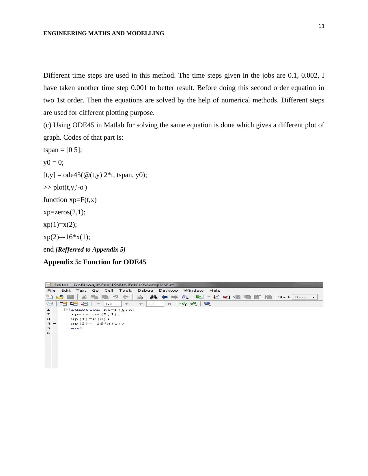
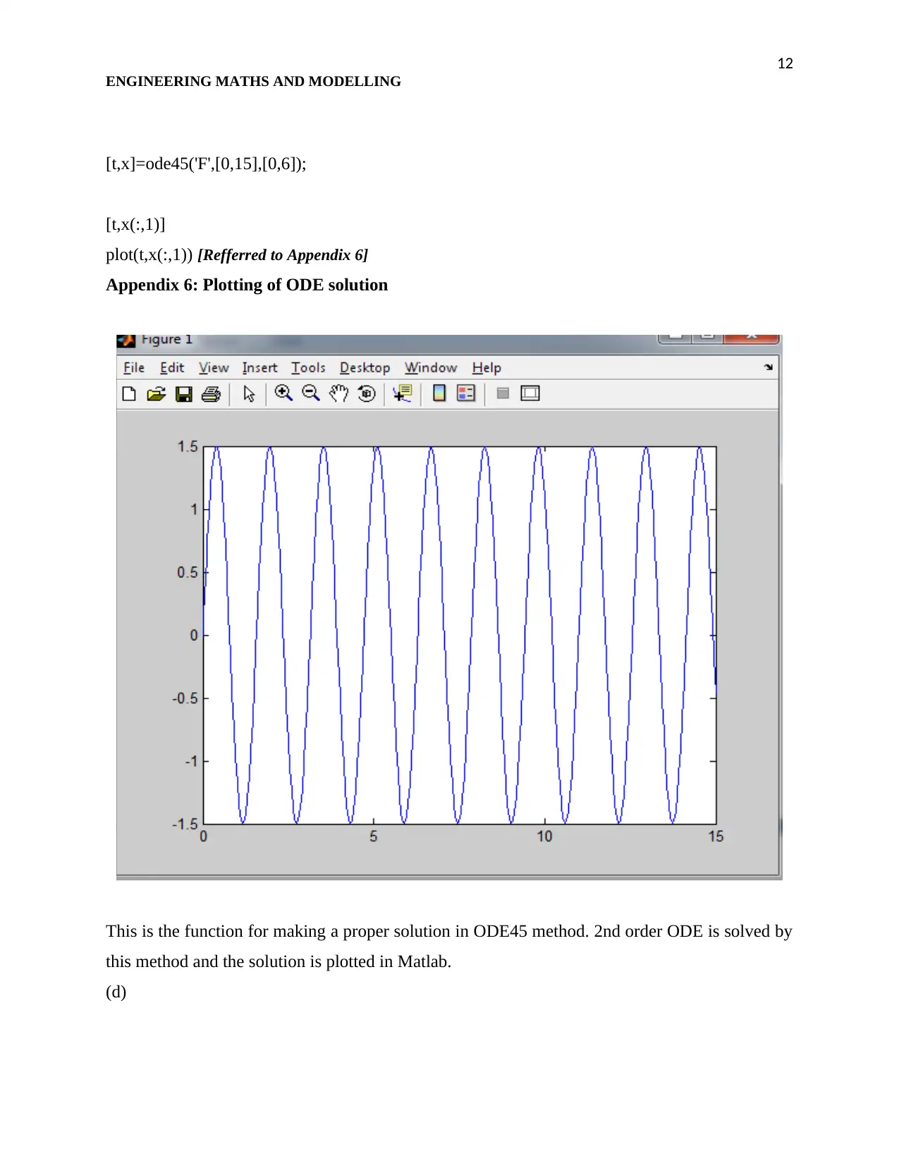
This report provides a comprehensive analysis of a spring-mass-damper (MSD) system, a fundamental concept in engineering, particularly relevant to civil engineering applications. The study begins with deriving the governing equations of motion, which are then solved using both analytical and numerical methods, including Euler's method and the ODE45 solver in Matlab. The report investigates the impact of various parameters, such as mass, spring constant, and damping coefficients, on the system's behavior, including displacement, velocity, and acceleration. Key findings are presented, highlighting the effects of different initial conditions and the influence of damping on the harmonic motion of the system. The report also includes Matlab code and plots, demonstrating the practical application of these methods. By comparing the results obtained from different approaches, the study offers insights into the accuracy and efficiency of each method. The analysis extends to the effects of damping, changing the initial conditions, and varying mass and spring constants on the solution. This coursework consolidates the knowledge of differential equations and their application in modeling and investigating the behavior of vibrating systems, ultimately providing a foundation for understanding more complex multi-component systems, like real-world structures, through the extension of MSD approaches.
Document Page
ENGINEERING MATHS AND MODELLING
tabler-icon-diamond-filled.svg

Paraphrase This Document

Need a fresh take? Get an instant paraphrase of this document with our AI Paraphraser
Document Page
2
ENGINEERING MATHS AND MODELLING
Executive summary
Matlab is a useful tool for solving complex equations easily. Governing equation of the spring-
mass system is derived by the help of analytical method for the single and double spring-mass
system. It follows Hook's law and Newton's law of motion. Spring mass system follows a
harmonic motion which is also dependable on various factors. The variables on which
displacement is dependent on are mass, spring constant, initial conditions, stiffness, damping
factor, and many others. The effect of those on displacement is shown by the help of graphs and
plotting. Symbolic, Analytical, Euler, ODE45 methods are used in solving the governing motion
equations of spring-mass system in this study. Different values of the independent variables are
taken in here for finding proper analysis. The study reflects the use of those equations in
different methods and also shows the different results found in different methods by the use of
Matlab. Findings regarding the entire topic are mentioned clearly in this report which will help to
get a clear idea about the spring-mass-damping system.
Document Page
3
ENGINEERING MATHS AND MODELLING
Table of Contents
Introduction......................................................................................................................................4
Question 1........................................................................................................................................4
Key findings.................................................................................................................................9
Question 2......................................................................................................................................10
Key findings...............................................................................................................................18
Question 3......................................................................................................................................20
Key findings...............................................................................................................................33
Conclusion.....................................................................................................................................34
Reference List................................................................................................................................35
Appendices....................................................................................................................................38
Document Page
4
ENGINEERING MATHS AND MODELLING
Introduction
There are many cases where the relation of motion can be shown with respect to time. Spring
mass system is an example of harmonic motion. It follows Hook's law and Newton's law of
motion. Displacement, velocity, and acceleration can be found of any motion by the help of those
laws. In order to get the solution, we need to solve differential equations. In this study, we will
discuss various methods of solving differential equations. Analytical, Euler, ODE45, numerical
methods are used in this study for solving the governing equation of spring damping system.
Matlab helps us in solving any equation correctly and also in a quick process. The processes,
codes, and methods are required in performing a Matlab program. This study will help in
deriving and solving the governing equation for the spring-mass-damping system and also will
help to analyze the key findings during solving by the use of Matlab.
Question 1
a)
Fig 1: Spring mass damping system
(Source: http://ctms.engin.umich.edu/CTMS/index.php?
example=Introduction&section=SystemModeling)
(i) Governing equation describes about the change of unknown variables with change of known
ones. There is governing equations related to different motions. In case of this spring, a mass of
m is held there by MSD. Force F is applied on it for oscillating purpose (Harris, 2017). Force of
tabler-icon-diamond-filled.svg

Paraphrase This Document

Need a fresh take? Get an instant paraphrase of this document with our AI Paraphraser
Document Page
5
ENGINEERING MATHS AND MODELLING
the damper is given, where b is damping constant. Spring constant k is given there. Deriving a
governing equation, below steps can be used:
F= ma;
a= dx2/dt2;
Considering gravity force, spring force and damping force in this:
mg - k(s+x) = F - b * dx/dt;
mg - k(s+x) = mdx2/dt2 - b * dx/dt;
This is the governing equation for the given figure.
(ii) The conditions here are given for the figure where the governing equation is needed to be
solved. The conditions provided are;
F= 0, m=10 kg, k= 160N/ m, b= 0 N s/m;
x(0) = 0, dx/dt |x=0 = 6;
Gravity force is taken here as negligible. So, force due to gravity is eliminated in the equation.
Besides, spring force is also taken as zero for ease in solution (Cárcamo, Gómez & Fortuny,
2016).
mdx2/dt2 + kx= 0;
dx2/dt2 + (k/m)x = 0;
dx2/dt2 + (160/10)x = 0;
dx2/dt2 + 16x = 0;
Taking the ODE for solution:
D2+ 16= 0;
D= ± 4;
Appendix 1: Symbolic form of solution in Matlab
Document Page
6
ENGINEERING MATHS AND MODELLING
x(t) = c1 cost 4t + c2 sin 4t;
As, x(0) = 0;
0 = c1 cost 0 + c2 sin 0 = c1 ;
So, x(t) = c2 sin 4t;
x’(t) = 4c2 cos 4t;
As, dx/dt |x=0 = 6, 4c2 = 6
c2 = 3/2= 1.5;
So, x(t) = 1.5 sin 4t;
This is the solution for governing equation in this case.
(iii) By the help of Matlab symbolic software it is noted that above solution is correct. The
command history regarding that is shown below: [Referred to Appendix 1]
syms x t;
dsolve('D2y+16*y=0')
syms x t;
dsolve('D2x+16*x=0', 'Dx(0)=6', 'x(0)=0', 't')
(iv) Plotting of curves with respect to displacement and time is done in Matlab using below
codes: [Referred to Appendix 2]
Appendix 2: Displacement graph
Document Page
7
ENGINEERING MATHS AND MODELLING
tabler-icon-diamond-filled.svg

Paraphrase This Document

Need a fresh take? Get an instant paraphrase of this document with our AI Paraphraser
Document Page
8
ENGINEERING MATHS AND MODELLING
clear all;
>> close all;
>> t= 0:0.01:15;
>> x= 1.5*sin(4*t);
>> subplot(2,1,1);
>> plot(t,x);
(v) Adding the damping function will provide different result in this case. Damping coefficient is
taken as 4N s/m. This gives a different solution in this case (Chen et al. 2017). The solution
given in this case is done by the help of Matlab by code:
syms x t;
dsolve('D2x-4Dx+16*x=0', 'Dx(0)=6', 'x(0)=0', 't')
This gives the solution as:
x= 3/2*sin(4t)-1/4*cos(4t)+¼;
This makes a change in displacement as can be seen in displacement by plotting curve:
clear all;
close all;
t= 0:0.01:3;
x= 1.5*sin(4*t)-0.25*cos(4*t)+0.25;
clear all;
t= 0:0.01:15;
x= 3/2*sin(4*t)-1/4*cos(4*t)+1/4;
subplot (2,1,1);
plot(t,x); [Refferred to Appendix 3]
Appendix 3: Damping factor in solution
Document Page
9
ENGINEERING MATHS AND MODELLING
(b)
Euler’s method coding is done to plot the curves in Matlab. Codes used are:
clear all;
close all;
clc;
f=@(t,y)t+y;
t0=0;
y0=6;
h=0.001;
tn=1;
n=(tn-t0)/h;
T(1)=t(0);
Y(1)=y(0);
for i=2:n
Y(i)= Y(i-1)+ h*feval(f,T(i-1),Y(i-1));
T(i)=T(i-1)+h;
end
figure(1);
sol=dsolve('Dy=t+y','y(0)=6', 't');
y_exact= inline(vectorize(sol));
plot(T,y_exact(T),'b*-');
Document Page
10
ENGINEERING MATHS AND MODELLING
xlabel('t');
ylable('y(t)');
hold on;
plot (T, Y, 'ro-');
legend('Exact Solution', 'Approx. Solution') [Refferred to Appendix 4]
Appendix 4: Euler’s method solution
tabler-icon-diamond-filled.svg

Paraphrase This Document

Need a fresh take? Get an instant paraphrase of this document with our AI Paraphraser
Document Page
11
ENGINEERING MATHS AND MODELLING
Different time steps are used in this method. The time steps given in the jobs are 0.1, 0.002, I
have taken another time step 0.001 to better result. Before doing this second order equation in
two 1st order. Then the equations are solved by the help of numerical methods. Different steps
are used for different plotting purpose.
(c) Using ODE45 in Matlab for solving the same equation is done which gives a different plot of
graph. Codes of that part is:
tspan = [0 5];
y0 = 0;
[t,y] = ode45(@(t,y) 2*t, tspan, y0);
>> plot(t,y,'-o')
function xp=F(t,x)
xp=zeros(2,1);
xp(1)=x(2);
xp(2)=-16*x(1);
end [Refferred to Appendix 5]
Appendix 5: Function for ODE45
Document Page
12
ENGINEERING MATHS AND MODELLING
[t,x]=ode45('F',[0,15],[0,6]);
[t,x(:,1)]
plot(t,x(:,1)) [Refferred to Appendix 6]
Appendix 6: Plotting of ODE solution
This is the function for making a proper solution in ODE45 method. 2nd order ODE is solved by
this method and the solution is plotted in Matlab.
(d)
chevron_up_icon
1 out of 50
circle_padding
hide_on_mobile
zoom_out_icon
[object Object]