ENS5447 Propagation and Antennas Assignment Solution - Semester 2

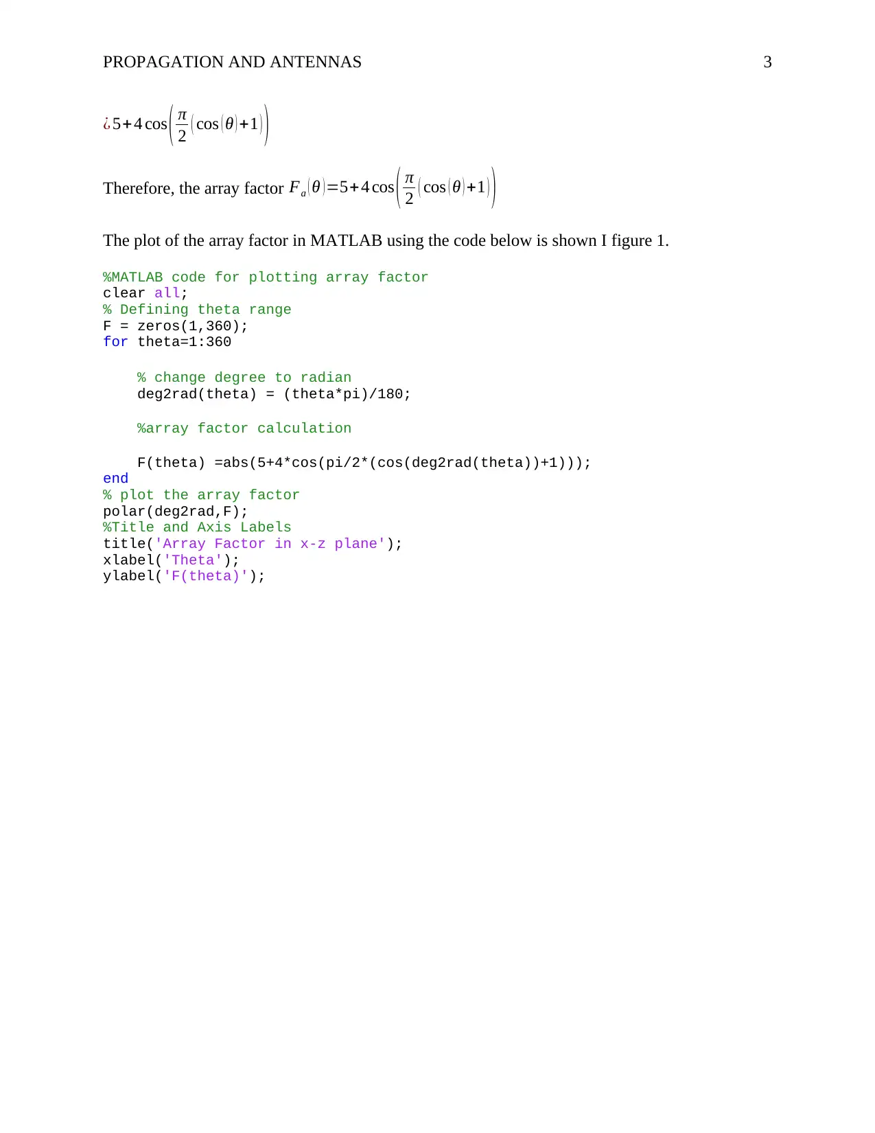
This assignment solution covers several key aspects of propagation and antennas. It begins with calculating the array factor for a two-element antenna array and plotting it using MATLAB. It then determines the normalized array factor for a six-element array, calculates the half-power beam width, and plots the array using MATLAB. The solution further explores the array factor for a three-element array, including simplification and MATLAB plotting. Additionally, it includes energy storage calculation within a defined cylindrical region using both analytical and numerical (MATLAB) methods, demonstrating comparable results. Finally, the assignment calculates the incremental phase delay and array factor for an eight-element array with a specified scan angle.

Running head: PROPAGATION AND ANTENNAS 1
Propagation and Antennas
Name
Institution

PROPAGATION AND ANTENNAS 2
Question 1
a0=1 , a1=2 , δ= π
2 , d= λ
4
The expression for an N-element antenna array factor is:
Fa ( θ ) =|∑
i=0
N−1
ai e j ψ 1
e jikdcos ( θ )
|
2
Since it is a two-element array, we substitute N=2 to get:
Fa ( θ ) =|∑
i=0
N−1
ai e j ψ 1
e jikdcos ( θ )
|
2
=|∑
i=0
2−1
ai e jψ1
e jikdcos ( θ )
|
2
=|∑
i=0
1
ai e j ψ1
e jikdcos ( θ )
|
2
¿|a0 e j ψ0
e j (0 )kdcos (θ ) +a1 e j ψ 1
e j(1)kdcos (θ )
|2
¿|a0 +a1 e j δ e j ( 2 π
λ ) dcos ( θ )
|
2
Substituting the values for a0 , a1 , δ ,∧dwe get:
Fa ( θ )=|1+2 e j ( π
2 ) e j ( 2 π
λ )( λ
4 )cos (θ )
|2
=|1+2 e j ( π
2 ) e j ( π
2 )cos (θ )
|2
¿|1+2 e j ( π
2 ) cos ( θ ) + j ( π
2 )|
2
=|1+2 e j ( π
2 ) ( cos ( θ ) +1 )
|
2
¿
|1+2 [ cos ( π
2 ( cos ( θ ) +1 ) ) + jsin ( π
2 ( cos ( θ ) +1 ) ) ]|
2
¿
|1+2 cos ( π
2 ( cos ( θ ) +1 ) )|2
+
|2 sin ( π
2 ( cos ( θ )+ 1 ))|2
¿ 1+4 cos ( π
2 ( cos ( θ ) +1 ) )+ 4 co s2
( π
2 ( cos ( θ ) +1 ) )+4 si n2
( π
2 ( cos ( θ )+1 ) )
¿ 1+4 cos ( π
2 ( cos ( θ ) +1 ) )+ 4 {co s2
( π
2 ( cos (θ ) +1 ) )+ si n2
( π
2 ( cos ( θ )+1 ) ) }
¿ 1+4 cos ( π
2 ( cos ( θ ) +1 ) )+ 4 (1)

PROPAGATION AND ANTENNAS 3
¿ 5+ 4 cos ( π
2 ( cos ( θ ) +1 ) )
Therefore, the array factor Fa ( θ ) =5+4 cos ( π
2 ( cos ( θ ) +1 ) )
The plot of the array factor in MATLAB using the code below is shown I figure 1.
%MATLAB code for plotting array factor
clear all;
% Defining theta range
F = zeros(1,360);
for theta=1:360
% change degree to radian
deg2rad(theta) = (theta*pi)/180;
%array factor calculation
F(theta) =abs(5+4*cos(pi/2*(cos(deg2rad(theta))+1)));
end
% plot the array factor
polar(deg2rad,F);
%Title and Axis Labels
title('Array Factor in x-z plane');
xlabel('Theta');
ylabel('F(theta)');

PROPAGATION AND ANTENNAS 4
Figure 1: MATLAB Array Factor Plot
Question 2
Array Factor , Fa ( γ' ) =
si n2
( N γ '
2 )
N2 si n2
( γ '
2 ) , N=number of elements
γ'=kdcos θ−kdcos θ0
but , δ=kdcos θ0 =0 due to equal phase excitation. Hence, γ' =kdcos θ
spacing, d = λ
2 ∧k= 2 π
λ

PROPAGATION AND ANTENNAS 5
Fa ( θ )=
si n2
( 6 × 2 π
λ × λ
2 cos θ
2 )
62 si n2
( 2 π
λ × λ
2 cos θ
2 ) = si n2 ( 3 π cos θ )
36 si n2
( π
2 cos θ )
Fa ( θ )= si n2 ( 3 π cos θ )
36 si n2
( π
2 cos θ )=
( sin (3 π cos θ )
6 sin ( π
2 cos θ ) )2
The MATLAB script for plotting the array is shown below.
%MATLAB code for plotting array factor
clear all;
% Defining theta range
F = zeros(1,360);
for theta=1:360
% change degree to radian
deg2rad(theta) = (theta*pi)/180;
%array factor calculation
F(theta)=abs((sin((3*pi*cos(deg2rad(theta))))/(6*sin(((pi/2)*cos(deg2rad(theta
))))))^2);
end
% plot the array factor
polar(deg2rad,F);
%Title and Axis Labels
title('Normalized Array Factor');
xlabel('Theta');
ylabel('F(theta)');
Figure 2 shows the normalized array factor plot in MATLAB.

PROPAGATION AND ANTENNAS 6
Figure 2: Normalized Array Plot
Half-power beam width
Fa ( θ )= si n2 ( 3 π cos θ )
36 si n2
( π
2 cos θ )= 1
2
2 si n2 ( 3 π cos θ )=36 si n2
( π
2 cos θ )
sin2 ( 3 π cos θ )=18 sin2
( π
2 cos θ )
sin2 ( 3 π cos θ )−18 sin2
( π
2 cos θ )=0
Solving the equation, we obtain:

PROPAGATION AND ANTENNAS 7
θ1=1.421 rad , θ2=1.721 rad ,θ3=4.562 ,∧θ4 =4.862
Half power beam width, β=θ2−θ1
¿ 1.721−1.421=0.3 rad
β=0.3 × 180 °
π =17.1887 °
Question 3
The three-array element alignment can be represented as:
The expression for an N-element antenna array factor is:
Fa ( θ ) =|∑
i=0
N−1
ai e j ψ 1
e jikdcos ( θ )
|
2
Since it is a three-element array, we substitute N=3 to get:

PROPAGATION AND ANTENNAS 8
Fa ( θ ) =
|∑
i=0
N−1
ai e j ψ 1
e jikdcos ( θ )
|
2
=
|∑
i=0
3−1
ai e jψ 1
e jikdcos ( θ )
|
2
=
|∑
i=0
2
ai e j ψ1
e jikdcos ( θ )
|
2
¿|∑
i=0
2
ai e jψ i
e ji ( 2 π
λ )( 3 λ
4 )cos (θ )
|2
=|∑
i=0
2
ai e j ψi
e ji ( 3 π
2 )cos (θ )
|2
In such a scenario, a0=1 , a1=2 ,∧a2=1.
Also, ψ0=−π
2 , ψ1=0 ,∧ψ2= π
2
Fa ( θ )=|a0 e j ψ0
e j 0 3 π
2 cos ( θ )
+a1 e j ψ 1
e j 1 3 π
2 cos (θ )
+ a2 e jψ 2
e j 2 3 π
2 cos (θ )
|2
Fa ( θ )=|e
− jπ
2 +2 e
j 3 π
2 cos ( θ )
+e
jπ
2 e j 3 πcos (θ )
|2
Fa ( θ )=|− j+ 2cos ( 3 π
2 cos ( θ ) )+ j 2 sin ( 3 π
2 cos ( θ ) )+ jcos ( 3 πcos ( θ ) ) −sin ( 3 πcos (θ ) )|2
¿ ¿ ¿
¿|2 cos ( 3 π
2 cos ( θ ) ) −sin ( 3 πcos ( θ ) )|
2
+¿ ¿
¿ 4 co s2
( 3 π
2 cos ( θ ) )+si n2 ( 3 πcos ( θ ) )−4 cos ( 3 π
2 cos ( θ ) )sin ( 3 πcos ( θ ) )+ co s2 ( 3 πcos (θ ) ) +4 cos ( 3 πcos ( θ ) ) sin ( 3 π
2 c
Upon further simplification we get:
Fa ( θ ) =4 +1+4 [ −cos ( 3 π
2 cos ( θ ) ) sin ( 3 πcos ( θ ) ) + cos ( 3 πcos ( θ ) ) sin ( 3 π
2 cos ( θ ) ) ] +1−2 [ cos ( 3 πcos ( θ ) ) +2 sin ( 3 π
2 c
¿ 6−4 [ sin ( 3 πcos ( θ ) −3 π
2 cos ( θ ) ) ] −2 [ cos ( 3 πcos ( θ ) ) +2sin ( 3 π
2 cos ( θ ) ) ]
¿ 6−4 sin ( 3 π
2 cos ( θ ) )−2 cos ( 3 πcos ( θ ) ) −4 sin ( 3 π
2 cos ( θ ) )
Therefore , the array factor , Fa ( θ )=6−8 sin (3 π
2 cos ( θ ) )−2 cos ( 3 πcos ( θ ) )
The MATLAB code for plotting the array is shown below.

PROPAGATION AND ANTENNAS 9
%MATLAB code for plotting array factor
clear all;
% Defining theta range
F = zeros(1,360);
for theta=1:360
% change degree to radian
deg2rad(theta) = (theta*pi)/180;
%array factor calculation
F(theta)=6-8*sin(1.5*pi*cos(deg2rad(theta)))-
2*cos(3*pi*cos(deg2rad(theta)));
end
% plot the array factor
polar(deg2rad,F);
%Title and Axis Labels
title('Array Factor');
xlabel('Theta');
ylabel('F(theta)');
Figure 3 shows the resulting plot.

PROPAGATION AND ANTENNAS 10
Figure 3: MATLAB plot
Question 4
E=5 ×104
ρ ap ⇒ E=|E |= 5 ×104
ρ V m−1
Energy stored = 1
2∭
V
ε0 E2 Vⅆ
ε 0=8.854 × 10−12
In cylindrical coordinates, Vⅆ =ρ d ρ d ϕ dz
Energy stored = 1
2 ∫
z =−2
2
∫
ϕ=0
2 π
∫
ρ=1
2
8.854 ×10−12 × ( 5× 104
ρ )2
ρ d ρ d ϕ dz
¿ 1
2 ×8.854 × 10−12 × 25 ×108
∫
z =−2
2
∫
ϕ=0
2 π
∫
ρ=1
2
1
ρ2 ρ d ρ d ϕ dz
¿ 1.10675 ×10−2
∫
z =−2
2
∫
ϕ=0
2 π
∫
ρ=1
2
1
ρ d ρ d ϕ dz
¿ 1.10675 ×10−2
∫
z =−2
2
∫
ϕ=0
2 π
|ln ( ρ )|ρ=1
2
d ϕ dz
¿ 1.10675 ×10−2
∫
z =−2
2
∫
ϕ=0
2 π
ln ( 2 ) d ϕ dz
¿ 1.10675 ×10−2 × ln ( 2 ) ∫
z=−2
2
|ϕ|ϕ=0
2 π
dz
¿ 1.10675 ×10−2 × ln ( 2 ) ∫
z=−2
2
2 π dz
¿ 1.10675 ×10−2 × ln ( 2 ) ×2 π ∫
z=−2
2
dz=1.10675 ×10−2 × ln ( 2 ) ×2 π |z|z=−2
2
¿ 1.10675 ×10−2 × ln ( 2 ) ×2 π × 4
¿ 1. 928 ×10−1=0.1928 Joules

PROPAGATION AND ANTENNAS 11
Similarly, we divide the region into small energy volume elements, compute the volume of each
segment, and then add all the small energies. We use MATLAB to evaluate the total energy
using the formula:
Total Energy stored= 1
2 ε0 ∑
k =1
N
∑
j=1
N
∑
i=1
N
E2 ρk , j ,i Δ ρ Δϕ Δ z
The MATLAB code for computing the total energy is shown below.
clc; %clear the command line
Epsilon_naught=8.854*10^-12; %use permitivity of free space
%define the upper and lower limits of the three variables
upper_bound_rho=2.0;lower_bound_rho=1.0;
upper_bound_phi=2*pi;lower_bound_phi=0;
upper_z=2;lower_z=-2;
rho_Steps=30; %initialize rho
drho=(upper_bound_rho-lower_bound_rho)/rho_Steps; %The rho increment
z_Steps=50; %initialize the discretization in the z direction
dz=(upper_z-lower_z)/z_Steps; %The z increment
phi_Steps=30; %initialize the phi
dphi=(upper_bound_phi-lower_bound_phi)/phi_Steps;%The step in the phi
direction
WE=0;%the total energy
for k=1:phi_Steps
for j=1:z_Steps
for i=1:rho_Steps rho=lower_bound_rho+0.5*drho+(i-1)*drho;%radius of volume
element
z=lower_z+0.5*dz+(j-1)*dz; %z of current volume element
phi=lower_bound_phi+0.5*dphi+(k-1)*dphi; %phi of current volume element
Magnitude_E=5e4/rho; %magnitude of electric field of current volume element
dV=rho*drho*dphi*dz; %volume of current element
dWE=0.5*Epsilono*Magnitude_E*Magnitude_E*dV;%energy stored in current element
WE=WE+dWE; %get contribution to the total energy
end
end
end %end the loops
display(WE)

PROPAGATION AND ANTENNAS 12
Figure 4: MATLAB solution
Hence, the two methods yield the same answer.
Question 5
8-element array
Incremental phase delay , δ=kdcos θ0
Where :
spacing, d = λ
2
Scan angle, θ0 =90 °+60 °=150 °
¿ k =2 π
λ
Incremental phase delay , δ=kdcos θ0= 2 π
λ × λ
2 × cos 150° =−0.866 π
δ=−0.866 π =−2.7206 rad
Incremental phase delay=−2.7206× 180 °
π =−155.8846 °