Statistics: Environmental Data Analysis - Assignment 11, HW 11

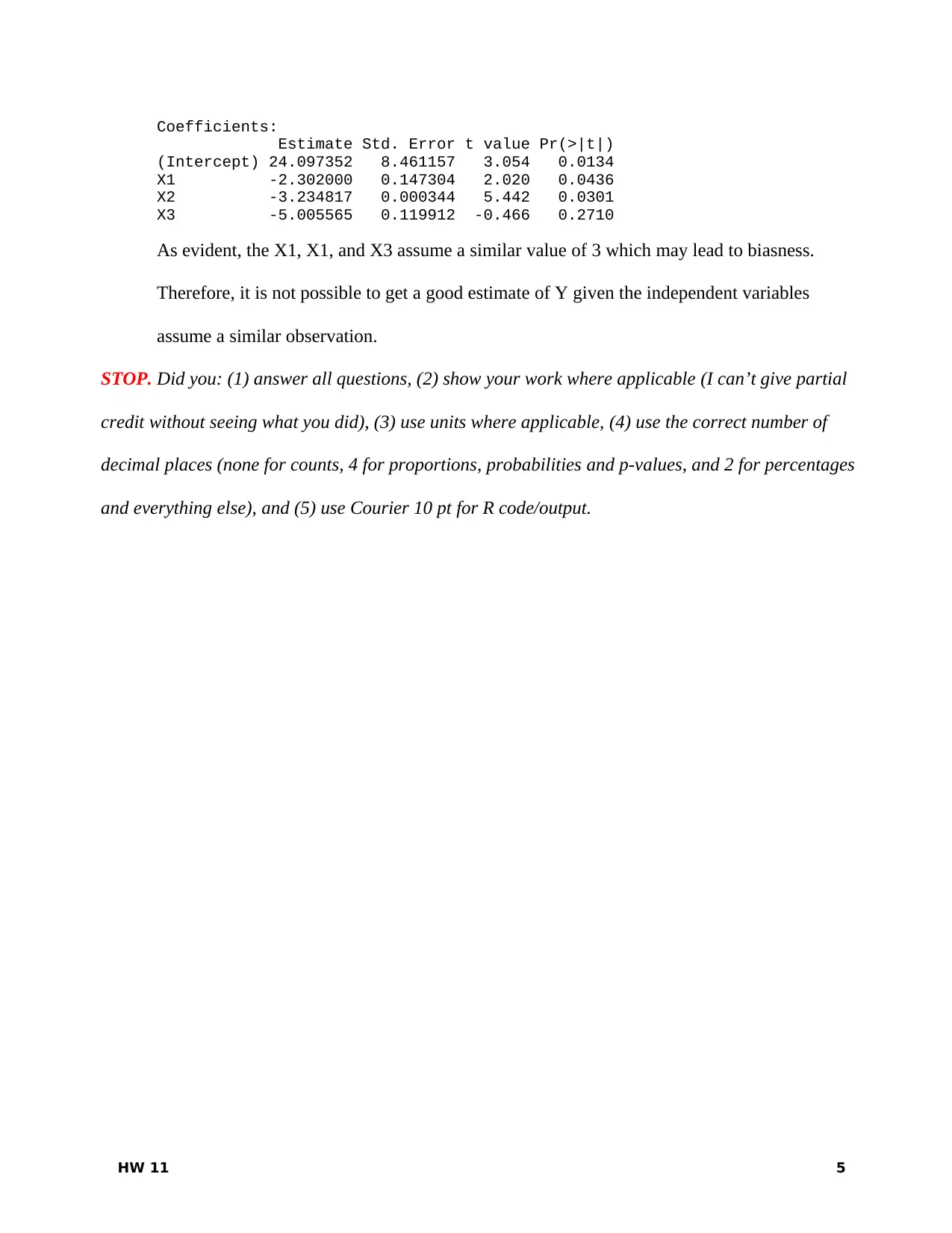
This assignment analyzes environmental data using statistical methods, focusing on regression analysis and model fitting. The student examines the relationship between children's heights and their parents' heights using Galton's data, employing R for model creation and diagnostic plot interpretation. The assignment explores multiple linear models, AIC, and the impact of variables on model performance. It involves fitting various models (father and mother, father only, mother only) and comparing their AIC values to determine the best fit. The student also investigates the impact of gender on the relationship between parent and child heights, along with identifying multiple linear models and interpreting model summaries. The assignment concludes by calculating estimates based on model coefficients and identifying potential issues in model interpretation.

Environmental Data Analysis - Assignment 11
Use the following for questions 1–6. In 1885, Francis Galton studied the relationship between the
height of adult children and their parents. This study is where the term “regression” comes from (see
Exercise 26 and Display 7.18 in the text). Galton measured the heights of 933 children from 205
families along with the heights of their parents. All measurements are in inches. Run the following
code to load the data:
require(Sleuth3)
data=ex0726
head(data)
1. Let’s start by fitting a full model with all of the variables and create the diagnostic plots.
Show your R output for the summary of this model and the diagnostic plots (if you want crop
out the bottom two plots that is OK).
m1=lm(data$Height~data$Father+data$Mother+data$Family)
windows()
par(mfrow=c(2,2))
plot(m1)
2. Are there any obvious problems with the fit of this model based on the diagnostic plots?
Explain.
As shown the residuals are randomly distributed around the 0 line thus exhibit a linear
relationship. However, there are residuals that stands out hence showing outliers in the data.
HW 11 1

3. Based on the model summary, one of the variables is not needed in the model? Which one and
explain why it is not useful (HINT – consider the nature of the variable).
lm(formula = data$Height ~ data$Father + data$Mother + data$Family)
Residuals:
Min 1Q Median 3Q Max
-9.081 -2.736 -0.208 2.772 11.652
Coefficients:
Estimate Std. Error t value Pr(>|t|)
(Intercept) 28.097649 12.466751 2.254 0.0244 *
data$Father 0.302389 0.149662 2.020 0.0436 *
data$Mother 0.281597 0.051742 5.442 6.73e-08 ***
data$Family -0.003065 0.006572 -0.466 0.6410
---
Signif. codes: 0 ‘***’ 0.001 ‘**’ 0.01 ‘*’ 0.05 ‘.’ 0.1 ‘ ’ 1
Residual standard error: 3.392 on 929 degrees of freedom
Multiple R-squared: 0.1055, Adjusted R-squared: 0.1026
F-statistic: 36.52 on 3 and 929 DF, p-value: < 2.2e-16
The model summary indicate that Family variable recorded a very high p value of 0.641;
besides, it acted a serial number to identify the families thus it is not needed and should be
dropped
4. The following code fits three models: father and mother, father only, and mother only; and
gives the AIC for each model. Which model is the best one to fit the data? Explain your
reasoning.
m2=lm(data$Height~data$Father+data$Mother)
m3=lm(data$Height~data$Father)
m4=lm(data$Height~data$Mother)
cbind(AIC(m2,m3,m4))
df AIC
m2 4 4931.290
m3 3 4964.342
m4 3 4994.666
Among the three models it is evident that m2 (father and mother) recorded the least AIC of
4931.290 thus it is the best one to fit the data.
5. What if we use only one parent to model the height of their child? Would it be a better model
to use only the father, only the mother, or should it be based on gender (i.e., use father’s
height with sons, and mother’s heights with daughters)? Run the following code which will
HW 11 2

subset the data into the female children (F) and the male children (M) and run separate models
based on their mothers and their fathers, along with the appropriate AICs. For each gender, is
it best to use the mother’s or the father’s height to model the children’s height? Explain your
reasoning.
F=data[which(data$Gender=="female"),]
M=data[which(data$Gender=="male"),]
M=M[1:453,]
m5=lm(F$Height~F$Mother)
m6=lm(F$Height~F$Father)
m7=lm(M$Height~M$Mother)
m8=lm(M$Height~M$Father)
cbind(AIC(m5,m6,m7,m8))
df AIC
m5 3 2022.682
m6 3 1974.628
m7 3 2120.929
m8 3 2099.343
The models above show that when modeling for the daughters’ height (F), m6 (Father)
recorded the lower AIC of 1974.628. Similarly, when modeling form sons’ height (M) m8
(Father) recorded a lower AIC of 2099.34. Therefore, it best to use the father’s height to
model the children’s height.
6. Can your conclusions from question #5 be supported by comparing m3 and m4? Explain.
As shown, m3 (Father) recorded a lower AIC of 4964.342 thus supporting a conclusion in part
6 to use the fathers height to model children’s height.
7. Which of the following model(s) is/are not a multiple linear model(s)? Explain why not.
As evident, in model A variable X is raised to 2 (X2, squared) thus it is model is not multiple
linear. Similarly, in model D is raised to another variable Xx3 thus it is not a multiple linear
model.
HW 11 3

8. Consider the information in Exercise 10 & Display 9.16 (p. 262 in the text). Looking at the p-
values, we see that each of the variables is significantly different from zero (and therefore
necessary in the model). Now pretend that “Social Class” had a p-value of 0.13. This would
suggest that the variable could be dropped. If we eliminate Social Class from the model, will
the estimated coefficients and p-values of the remaining variables remain the same or will
they change? Explain your reasoning.
Notably, by removing the non-significant variable the coefficients of the model improve;
besides, p-value changes but they coefficients will remain significant. Therefore, by removing
Social Class the model improves (estimate coefficients and p-values change) but they will be
significant.
9. Consider the following model summary. Estimate Y when X1 = 3, X2 = 2.2, and X3 = 0.3
(Use 2 decimal places rather than 6).
summary(m9)
Call:
lm(formula = Y ~ X1 + X2 + X3)
Coefficients:
Estimate Std. Error t value Pr(>|t|)
(Intercept) 21.097352 9.461157 3.254 0.0144
X1 2.302000 0.147304 2.020 0.0436
X2 3.234817 0.000344 5.442 0.0301
X3 -1.005565 0.009912 -3.466 0.0110
Y =21.097+2.302 X1+3.234 X2 – 1.006 X3
Y =21.10+2.30∗3+3.2 4∗2.2 – 1.0 1∗0.3
¿ 21.10+6.90+7.12−0.30=34.82
10. Consider the following model summary. It is not possible to get a good estimate of Y when
X1 = 3, X2 = 3, and X3 = 3. Why not?
summary(m10)
Call:
lm(formula = Y ~ X1 + X2 + X3)
HW 11 4

Coefficients:
Estimate Std. Error t value Pr(>|t|)
(Intercept) 24.097352 8.461157 3.054 0.0134
X1 -2.302000 0.147304 2.020 0.0436
X2 -3.234817 0.000344 5.442 0.0301
X3 -5.005565 0.119912 -0.466 0.2710
As evident, the X1, X1, and X3 assume a similar value of 3 which may lead to biasness.
Therefore, it is not possible to get a good estimate of Y given the independent variables
assume a similar observation.
STOP. Did you: (1) answer all questions, (2) show your work where applicable (I can’t give partial
credit without seeing what you did), (3) use units where applicable, (4) use the correct number of
decimal places (none for counts, 4 for proportions, probabilities and p-values, and 2 for percentages
and everything else), and (5) use Courier 10 pt for R code/output.
HW 11 5