Environmental Engineering: Diffusion Equation Solution and Analysis

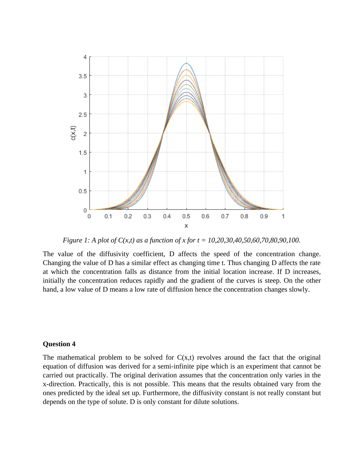
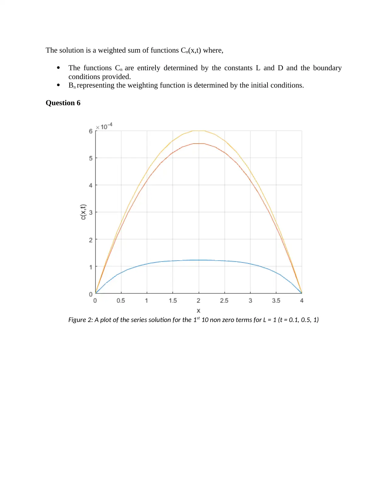
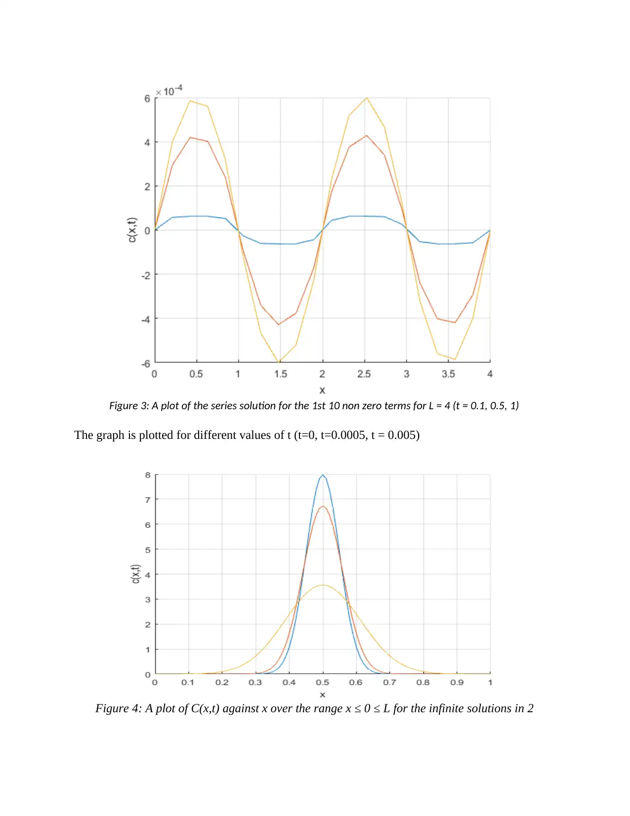
This assignment provides a detailed analysis and solution to the diffusion equation, focusing on pollutant distribution in a pipe. The solution explores various aspects, including the concentration of the pollutant as a function of time and space, with different initial conditions. It covers the derivation of the equation, solving for C(x,t) using different methods, and analyzing the impact of the diffusivity coefficient, D, on the rate of concentration change. The assignment addresses both semi-infinite and finite pipe scenarios, discussing the limitations of the original derivations and the practical implications of the solutions. Furthermore, it examines the effects of periodic functions to define the pollutant concentration, considering the impact of angular frequency on diffusion. The assignment includes plots and graphs to illustrate the concentration profiles under different conditions.

SOLUTION OF THE DIFFUSION EQUATION
Question 1
∂C
∂ t = D ∂2 C
∂ x2
The mathematical problem being solved concerns the distribution of the pollutant in the pipe as a
function of time and space with the initial conditions such as the concentration of the pollutant
being specified.
Solution of C(x,t)
Let C(x,t) = M(x)N(t) , differentiating C(x,t) with respect to t and x respectively we get,
∂C
∂ t = M dN
dt and ∂2 C
∂ x2 = M d2 M
d x2
We have M dN
dt = D d2 M
d x2 N hence dN
dt /DN = d2 M
d x2 /M = k
We obtain two ordinary differential equations from above,
d2 M
d x2 – kM = 0 and dN
dt – kDN = 0
Next we solve for M,
With k>0, the general solution is M(x) = Ceμx+ Deμx
Applying the boundary conditions, C+D = 0, Aeμx + Beμx =0 and therefore A = B = 0
With k = -p2
M(x) = C cos(px) + D sin(px) and the conditions at the boundary give,
M(0) = A = 0, M(L) = Dsin(pL) = 0 hence sin(pL) = 0 therefore Mn(x) = sin( nπ
L )x
Next we solve for N,
We have p = nπ
L and define λn = n Dπ
L , hence dN
dt + ¿λn2N = 0
The general solution is then given by: Nn (t) = Bne− λn 2
The solution to the one dimensional diffusion equation is thus: C(x,t) = ∑
n =1
∞
Cn ( x , t )= ∑
n =1
∞
Bn e−λ n 2
sin( nπ
L )x

The initial condition is C(x,0) ¿ ∑
n=1
∞
Bn sin( nπ
L )x = C(x), Bn = 2
L∫
0
L
C ( x ) sin( nπ
L )x dx
Question 2
From the equation, ∂C
∂ t = D ∂2 C
∂ x2 with C(x,0) = 0, C(0,t) = Co
Converting the diffusion equation into frequency domain yields;
∂ F (x , s)
∂ x = D ∂2 F ( x , s)
∂ x2 and F(0,s) = C o
s
F(x,s) = C o
s exp (-√s / Dx)
From inverse Laplace transform tables, L [ erfc ( a
2 √ t ) ] = exp ¿ ¿
Therefore, C(x,t) = Co erfc ( x
2 √Dt )
Question 3

Figure 1: A plot of C(x,t) as a function of x for t = 10,20,30,40,50,60,70,80,90,100.
The value of the diffusivity coefficient, D affects the speed of the concentration change.
Changing the value of D has a similar effect as changing time t. Thus changing D affects the rate
at which the concentration falls as distance from the initial location increase. If D increases,
initially the concentration reduces rapidly and the gradient of the curves is steep. On the other
hand, a low value of D means a low rate of diffusion hence the concentration changes slowly.
Question 4
The mathematical problem to be solved for C(x,t) revolves around the fact that the original
equation of diffusion was derived for a semi-infinite pipe which is an experiment that cannot be
carried out practically. The original derivation assumes that the concentration only varies in the
x-direction. Practically, this is not possible. This means that the results obtained vary from the
ones predicted by the ideal set up. Furthermore, the diffusivity constant is not really constant but
depends on the type of solute. D is only constant for dilute solutions.

Question 5
Let c(x,t) = P(x)Q(t), then P'' – λP = 0 for 0<x<L and P'' (0) = P''(L)
We consider three cases for λ;
Case (i) λ > 0, let λ = k2
Therefore, P'' – k2P = 0, this equation has the general solution P = A cosh (kx) + B sinh (kx)
Taking the derivative we obtain P' = Ak sinh (kx) + Bk cosh (kx)
If we apply the boundary conditions at x=0, x=L we get;
P' = Ak×0 + Bk×1 = 0 and P' = Ak sinh (kL) + Bk cosh (kL) = 0 with the solution A = B = 0
Case (ii) λ = 0,
Then P'' = 0 and P = Ax + B
Applying boundary conditions gives; P'(0) = A = 0 and P'(L) = A = 0
Case (iii) λ < 0, let λ = -k2 for k > 0
We have, P'' + k2P = 0 which has the solution, P = A cos (kx) + B sin (kx)
Taking the derivative yields: P' = -Ak sin (kx) + Bk cos (kx) and from P'(0) = 0 we get;
P'(0) = -Ak×0 + Bk×1 = 0, since k>0, B = 0.
Applying P'(L) = 0 yields P'(L) = = -Ak sin (kL) = 0
Sin (kL) = 0 or k = nπ
L for n = 0, 1, 2,..
Pn(x) = A cos ( nπx
L )
The general solution is thus, c(x,t) = ∑
n=0
∞
Bn exp [ −( nπx
L )
2
kt ]cos ( nπx
L )
The above equation can be written as: C(x,t) = ∑
n =1
∞
BnCn(x,t)

The solution is a weighted sum of functions Cn(x,t) where,
 The functions Cn are entirely determined by the constants L and D and the boundary
conditions provided.
 Bn representing the weighting function is determined by the initial conditions.
Question 6
Figure 2: A plot of the series solution for the 1st 10 non zero terms for L = 1 (t = 0.1, 0.5, 1)

Figure 3: A plot of the series solution for the 1st 10 non zero terms for L = 4 (t = 0.1, 0.5, 1)
The graph is plotted for different values of t (t=0, t=0.0005, t = 0.005)
Figure 4: A plot of C(x,t) against x over the range x ≤ 0 ≤ L for the infinite solutions in 2

We observe that for very short times, the pollutant concentration maintains its Gaussian shape as
predicted by the diffusion equation if there are no boundaries. However, the concentration finally
spreads out as evident from the graphs.
Question 7
Since in this case a periodic function is used to define the pollutant concentration in the pipe, the
mathematical problem to be solved involves determining the level of concentration of the
pollutant at any given time throughout the pipe. It is assumed that pollutant diffusion across the
pipe walls is small enough such that it can be ignored.
From the equation, ∂C
∂ t = D ∂2 C
∂ x2 with C(x,0) = 0, C(0,t) = Co cos(ωt) + Co
Converting the diffusion equation into frequency domain yields;
∂ F (x , s)
∂ x = D ∂2 F ( x , s)
∂ x2 and F(0, s) = C o cos (ωt )+C o
s
F(x, s) = C o cos (ωt )+C o
s exp (- √ s / Dx)
From inverse Laplace transform tables, L [ erfc ( a
2 √ t ) ] = exp ¿ ¿
Therefore, C(x,t) = Co cos(ωt) + Co erfc ( x
2 √Dt )
Let the solution of the equation be given as: u(x, t)=X(x)T(t) is assumed, where X is a function
of x only and T is a function of t only. If the trial solution is simplified to u=XT, then This
equation can be written as:
∂ u
∂ x = X'T, ∂2 u
∂ x2 = X''T and ∂u
∂ t = XT'
Substituting into the partial differential equation,
∂C
∂ t = D ∂2 C
∂ x2 gives X''T = DXT'
Separating the variables we obtain: X ' '
X = D T '
T

Next we define –p2 (a constant) = X ' '
X = D T '
T
If –p2 = X ' '
X then X'' = –p2X or X'' + p2X = 0 which a solution of the form: X =Acos px
+Bsin px
Similarly if –p2 = D T '
T then T '
T = – p 2
D and integrating with respect to t gives:
∫ T '
T dt = ∫ – p 2
D dt from which T = – p 2
D t + c1, The left hand integral is
obtained by algebraic substitution.
If ln T = – p 2
D t + c1 then T = e
– p 2
D t +c 1 that is, T = k e
– p 2
D t where k = ec 1
Hence C(x,t) = XT = [A cos px +B sin px]ke
– p 2
D t that is, C(x,t) = [P cos px +Q sin
px]e
– p 2
D t where P = Ak and Q = Bk
Applying the boundary conditions C(0, t) = Co cos(ωt) + Co gives,
Co cos(ωt) + Co = [P cos px +Q sin px]e
– p 2
D t
C(x,t) = A (x) cos (ωt) + B (x) sin (ωt) + Co
Question 8

Figure 5: A plot of C(x,t) versus x for ω = 4
Figure 6: A plot of C(x,t) versus x for ω = 1
The two graphs for ω = 1 and ω = 4 are shown above. We observe that, as the angular frequency
increases, the graph becomes narrower and the value of C(x,t) falls sharply as the distance from
the midpoint increases. However the general shape of the plot remains the same. We conclude
that a higher angular frequency speeds up diffusion which makes the initial concentration reduce
rapidly.