Epidemiology and Biostatistics Assignment: Analysis of Data

This assignment on epidemiology and biostatistics covers various aspects of data analysis and interpretation. The student addresses questions on incidence and prevalence, calculating cumulative frequency and incidence rates for a disease. The assignment also delves into relative risk, assessing the impact of alcohol consumption on mortality and analyzing the relationship between cigarette smoking and lung cancer. Furthermore, it explores confounding variables, identifying factors such as age, health status, and smoking habits that can influence study outcomes. The student also examines the influence of age on the risk of lung cancer and discusses potential confounders in studies related to CABG mortality and the effects of magnetic fields. Finally, the assignment touches upon experimental mortality and instrumentation as internal threats, along with a discussion of confounding variables like BMI and depression, providing insights into the complexities of epidemiological research.

Running head: EPIDEMIOLOGY AND BIOSTATISTICS 1
Epidemiology and Biostatistics
Student’s Name
University Affiliation

EPIDEMIOLOGY AND BIOSTATISTICS 2
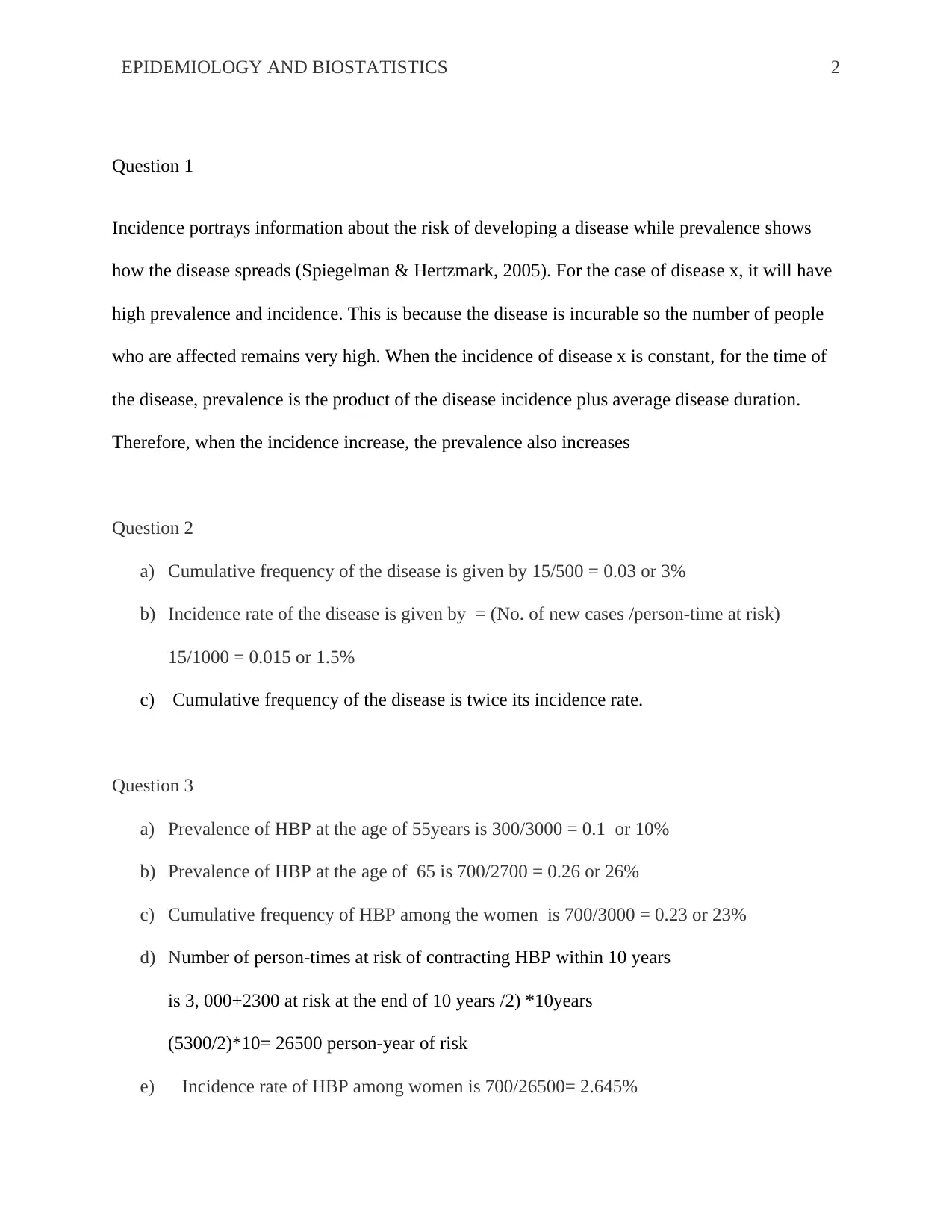
Question 1
Incidence portrays information about the risk of developing a disease while prevalence shows
how the disease spreads (Spiegelman & Hertzmark, 2005). For the case of disease x, it will have
high prevalence and incidence. This is because the disease is incurable so the number of people
who are affected remains very high. When the incidence of disease x is constant, for the time of
the disease, prevalence is the product of the disease incidence plus average disease duration.
Therefore, when the incidence increase, the prevalence also increases
Question 2
a) Cumulative frequency of the disease is given by 15/500 = 0.03 or 3%
b) Incidence rate of the disease is given by = (No. of new cases /person-time at risk)
15/1000 = 0.015 or 1.5%
c) Cumulative frequency of the disease is twice its incidence rate.
Question 3
a) Prevalence of HBP at the age of 55years is 300/3000 = 0.1 or 10%
b) Prevalence of HBP at the age of 65 is 700/2700 = 0.26 or 26%
c) Cumulative frequency of HBP among the women is 700/3000 = 0.23 or 23%
d) Number of person-times at risk of contracting HBP within 10 years
is 3, 000+2300 at risk at the end of 10 years /2) *10years
(5300/2)*10= 26500 person-year of risk
e) Incidence rate of HBP among women is 700/26500= 2.645%

EPIDEMIOLOGY AND BIOSTATISTICS 3
Question 4
a) Period prevalence of hypertension is 1500/30000= 5%
b) Cumulative incidence of hypertension is 600/30000= 0.02
c) Incidence rate of hypertension is 600/36000= 1.7%
d) Cumulative incidence of hypertension is much higher compared to the incidence rate due
to an increase in population and the number of hypertension incidences.
Question 5
The study report with relative risk of 1.8 at 95 percent confidence interval of 1.6–2.0 for the
link between alcohol consumption and cancer is ideal since it shows precise plus statistically
significant estimate because the CI is narrow and doesn’t include 1.0 (Jekel et al., 2007). Also
the 1.8 RR indicates an 80% increases relative risk of cancer due to alcohol consumption.
Question 6
a)
Alcohol consumption group
Never Occasional Light Medium Heavy
At
danger
subjects
466 1845 2544 2042 832
No. of
deaths
126 439 654 512 62

EPIDEMIOLOGY AND BIOSTATISTICS 4
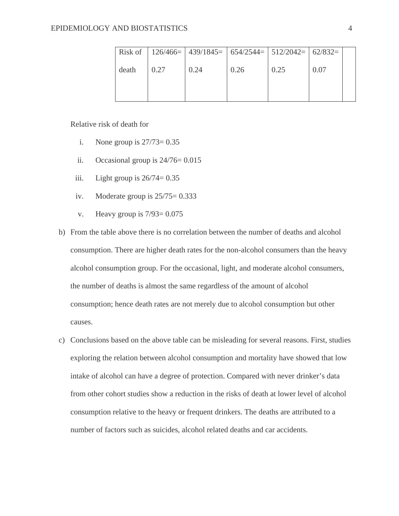
Risk of
death
126/466=
0.27
439/1845=
0.24
654/2544=
0.26
512/2042=
0.25
62/832=
0.07
Relative risk of death for
i. None group is 27/73= 0.35
ii. Occasional group is 24/76= 0.015
iii. Light group is 26/74= 0.35
iv. Moderate group is 25/75= 0.333
v. Heavy group is 7/93= 0.075
b) From the table above there is no correlation between the number of deaths and alcohol
consumption. There are higher death rates for the non-alcohol consumers than the heavy
alcohol consumption group. For the occasional, light, and moderate alcohol consumers,
the number of deaths is almost the same regardless of the amount of alcohol
consumption; hence death rates are not merely due to alcohol consumption but other
causes.
c) Conclusions based on the above table can be misleading for several reasons. First, studies
exploring the relation between alcohol consumption and mortality have showed that low
intake of alcohol can have a degree of protection. Compared with never drinker’s data
from other cohort studies show a reduction in the risks of death at lower level of alcohol
consumption relative to the heavy or frequent drinkers. The deaths are attributed to a
number of factors such as suicides, alcohol related deaths and car accidents.

EPIDEMIOLOGY AND BIOSTATISTICS 5
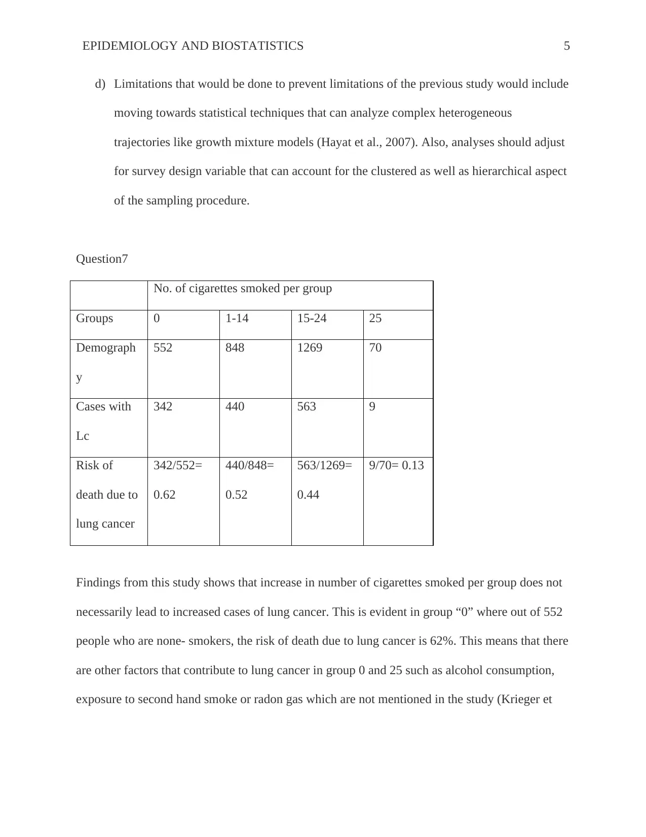
d) Limitations that would be done to prevent limitations of the previous study would include
moving towards statistical techniques that can analyze complex heterogeneous
trajectories like growth mixture models (Hayat et al., 2007). Also, analyses should adjust
for survey design variable that can account for the clustered as well as hierarchical aspect
of the sampling procedure.
Question7
No. of cigarettes smoked per group
Groups 0 1-14 15-24 25
Demograph
y
552 848 1269 70
Cases with
Lc
342 440 563 9
Risk of
death due to
lung cancer
342/552=
0.62
440/848=
0.52
563/1269=
0.44
9/70= 0.13
Findings from this study shows that increase in number of cigarettes smoked per group does not
necessarily lead to increased cases of lung cancer. This is evident in group “0” where out of 552
people who are none- smokers, the risk of death due to lung cancer is 62%. This means that there
are other factors that contribute to lung cancer in group 0 and 25 such as alcohol consumption,
exposure to second hand smoke or radon gas which are not mentioned in the study (Krieger et

EPIDEMIOLOGY AND BIOSTATISTICS 6
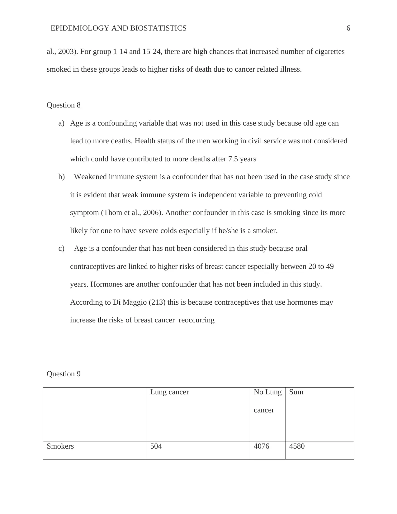
al., 2003). For group 1-14 and 15-24, there are high chances that increased number of cigarettes
smoked in these groups leads to higher risks of death due to cancer related illness.
Question 8
a) Age is a confounding variable that was not used in this case study because old age can
lead to more deaths. Health status of the men working in civil service was not considered
which could have contributed to more deaths after 7.5 years
b) Weakened immune system is a confounder that has not been used in the case study since
it is evident that weak immune system is independent variable to preventing cold
symptom (Thom et al., 2006). Another confounder in this case is smoking since its more
likely for one to have severe colds especially if he/she is a smoker.
c) Age is a confounder that has not been considered in this study because oral
contraceptives are linked to higher risks of breast cancer especially between 20 to 49
years. Hormones are another confounder that has not been included in this study.
According to Di Maggio (213) this is because contraceptives that use hormones may
increase the risks of breast cancer reoccurring
Question 9
Lung cancer No Lung
cancer
Sum
Smokers 504 4076 4580

EPIDEMIOLOGY AND BIOSTATISTICS 7
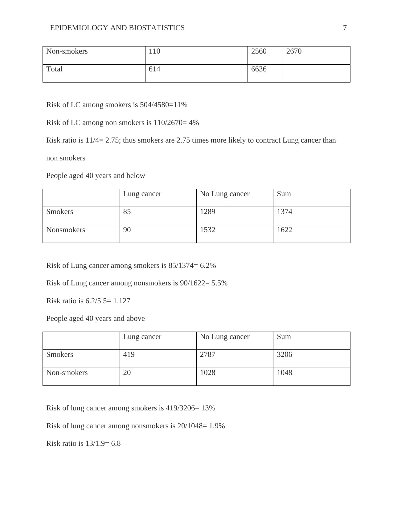
Non-smokers 110 2560 2670
Total 614 6636
Risk of LC among smokers is 504/4580=11%
Risk of LC among non smokers is 110/2670= 4%
Risk ratio is 11/4= 2.75; thus smokers are 2.75 times more likely to contract Lung cancer than
non smokers
People aged 40 years and below
Lung cancer No Lung cancer Sum
Smokers 85 1289 1374
Nonsmokers 90 1532 1622
Risk of Lung cancer among smokers is 85/1374= 6.2%
Risk of Lung cancer among nonsmokers is 90/1622= 5.5%
Risk ratio is 6.2/5.5= 1.127
People aged 40 years and above
Lung cancer No Lung cancer Sum
Smokers 419 2787 3206
Non-smokers 20 1028 1048
Risk of lung cancer among smokers is 419/3206= 13%
Risk of lung cancer among nonsmokers is 20/1048= 1.9%
Risk ratio is 13/1.9= 6.8

EPIDEMIOLOGY AND BIOSTATISTICS 8
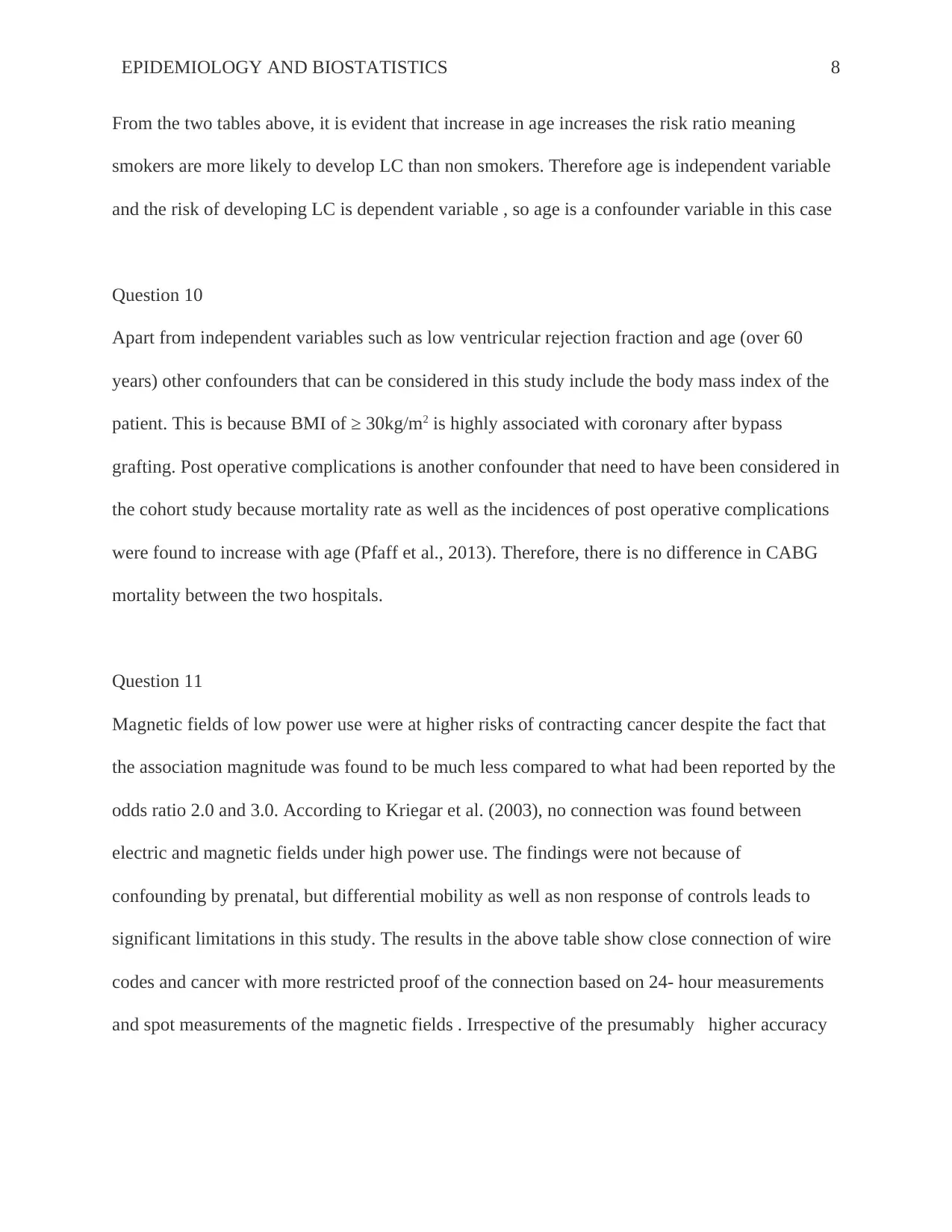
From the two tables above, it is evident that increase in age increases the risk ratio meaning
smokers are more likely to develop LC than non smokers. Therefore age is independent variable
and the risk of developing LC is dependent variable , so age is a confounder variable in this case
Question 10
Apart from independent variables such as low ventricular rejection fraction and age (over 60
years) other confounders that can be considered in this study include the body mass index of the
patient. This is because BMI of ≥ 30kg/m2 is highly associated with coronary after bypass
grafting. Post operative complications is another confounder that need to have been considered in
the cohort study because mortality rate as well as the incidences of post operative complications
were found to increase with age (Pfaff et al., 2013). Therefore, there is no difference in CABG
mortality between the two hospitals.
Question 11
Magnetic fields of low power use were at higher risks of contracting cancer despite the fact that
the association magnitude was found to be much less compared to what had been reported by the
odds ratio 2.0 and 3.0. According to Kriegar et al. (2003), no connection was found between
electric and magnetic fields under high power use. The findings were not because of
confounding by prenatal, but differential mobility as well as non response of controls leads to
significant limitations in this study. The results in the above table show close connection of wire
codes and cancer with more restricted proof of the connection based on 24- hour measurements
and spot measurements of the magnetic fields . Irrespective of the presumably higher accuracy

EPIDEMIOLOGY AND BIOSTATISTICS 9
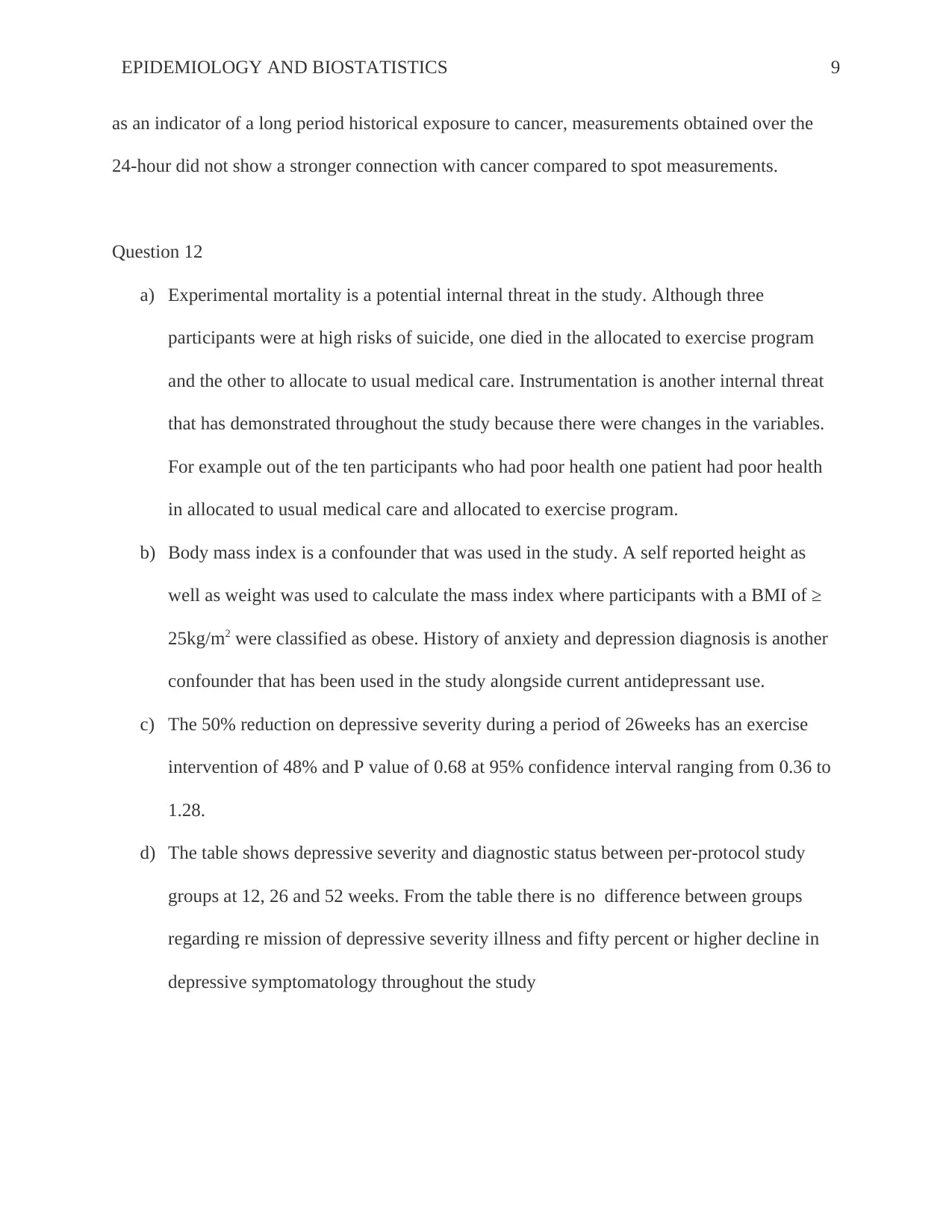
as an indicator of a long period historical exposure to cancer, measurements obtained over the
24-hour did not show a stronger connection with cancer compared to spot measurements.
Question 12
a) Experimental mortality is a potential internal threat in the study. Although three
participants were at high risks of suicide, one died in the allocated to exercise program
and the other to allocate to usual medical care. Instrumentation is another internal threat
that has demonstrated throughout the study because there were changes in the variables.
For example out of the ten participants who had poor health one patient had poor health
in allocated to usual medical care and allocated to exercise program.
b) Body mass index is a confounder that was used in the study. A self reported height as
well as weight was used to calculate the mass index where participants with a BMI of ≥
25kg/m2 were classified as obese. History of anxiety and depression diagnosis is another
confounder that has been used in the study alongside current antidepressant use.
c) The 50% reduction on depressive severity during a period of 26weeks has an exercise
intervention of 48% and P value of 0.68 at 95% confidence interval ranging from 0.36 to
1.28.
d) The table shows depressive severity and diagnostic status between per-protocol study
groups at 12, 26 and 52 weeks. From the table there is no difference between groups
regarding re mission of depressive severity illness and fifty percent or higher decline in
depressive symptomatology throughout the study

EPIDEMIOLOGY AND BIOSTATISTICS
10
REFERENCES
DiMaggio, C. (2013). ANOVA. In SAS for Epidemiologists (pp. 159-186). Springer New York.
DiMaggio, C. (2013). Introduction. In SAS for Epidemiologists (pp. 1-5). Springer New York.
Hayat, M. J., Howlader, N., Reichman, M. E., & Edwards, B. K. (2007). Cancer statistics, trends,
and multiple primary cancer analyses from the Surveillance, Epidemiology, and End
Results (SEER) Program. The oncologist, 12(1), 20-37.
Jekel, J. F., Katz, D. L., Elmore, J. G., & Wild, D. (2007). Epidemiology, biostatistics and
preventive medicine. Elsevier Health Sciences.
Krieger, N., Chen, J. T., Waterman, P. D., Rehkopf, D. H., & Subramanian, S. V. (2003).
Race/ethnicity, gender, and monitoring socioeconomic gradients in health: a comparison
of area-based socioeconomic measures—the public health disparities geocoding project.
American journal of public health, 93(10), 1655-1671.
Pfaff, J. J., Alfonso, H., Newton, R. U., Sim, M., Flicker, L., & Almeida, O. P. (2013).
ACTIVEDEP: a randomised, controlled trial of a home-based exercise intervention to
alleviate depression in middle-aged and older adults. Br J Sports Med, bjsports-2013.
Spiegelman, D., & Hertzmark, E. (2005). Easy SAS calculations for risk or prevalence ratios and
differences. American journal of epidemiology, 162(3), 199-200.
Thom, T., Haase, N., Rosamond, W., Howard, V. J., Rumsfeld, J., Manolio, T., ... & Lloyd-
Jones, D. (2006). Heart disease and stroke statistics--2006 update: a report from the
American Heart Association Statistics Committee and Stroke Statistics Subcommittee.
Circulation, 113(6), e85.