Epidemiology Assignment: Analysis of Health Data and Module Exercises

This assignment presents a comprehensive analysis of epidemiological data across several health-related modules. The first module examines Hepatitis B notifications in Australia from 1999 to 2019, discussing the declining trends and potential contributing factors like government interventions targeting indigenous populations and remote areas. The second module investigates the relationship between asthma wheeze prevalence and ambient atmospheric particulate matter (PM10) using both computerized and manual Pearson correlation calculations. Module three presents a chi-square analysis of the relationship between food practices (canteen vs. home-prepared) and student weight, suggesting improvements to school canteen food. The final module conducts a relative risk analysis to determine the impact of different foods on illness among bankers, identifying cream of mushroom soup as having the most significant risk of food poisoning. The assignment also includes a critique and revision of poorly designed interview questions, offering improved alternatives for data collection.

Running head: EPIDEMIOLOGY
Epidemiology
Name of the Student
Name of the University
Author note

1EPIDEMIOLOGY
Module exercise 2
Part 1:
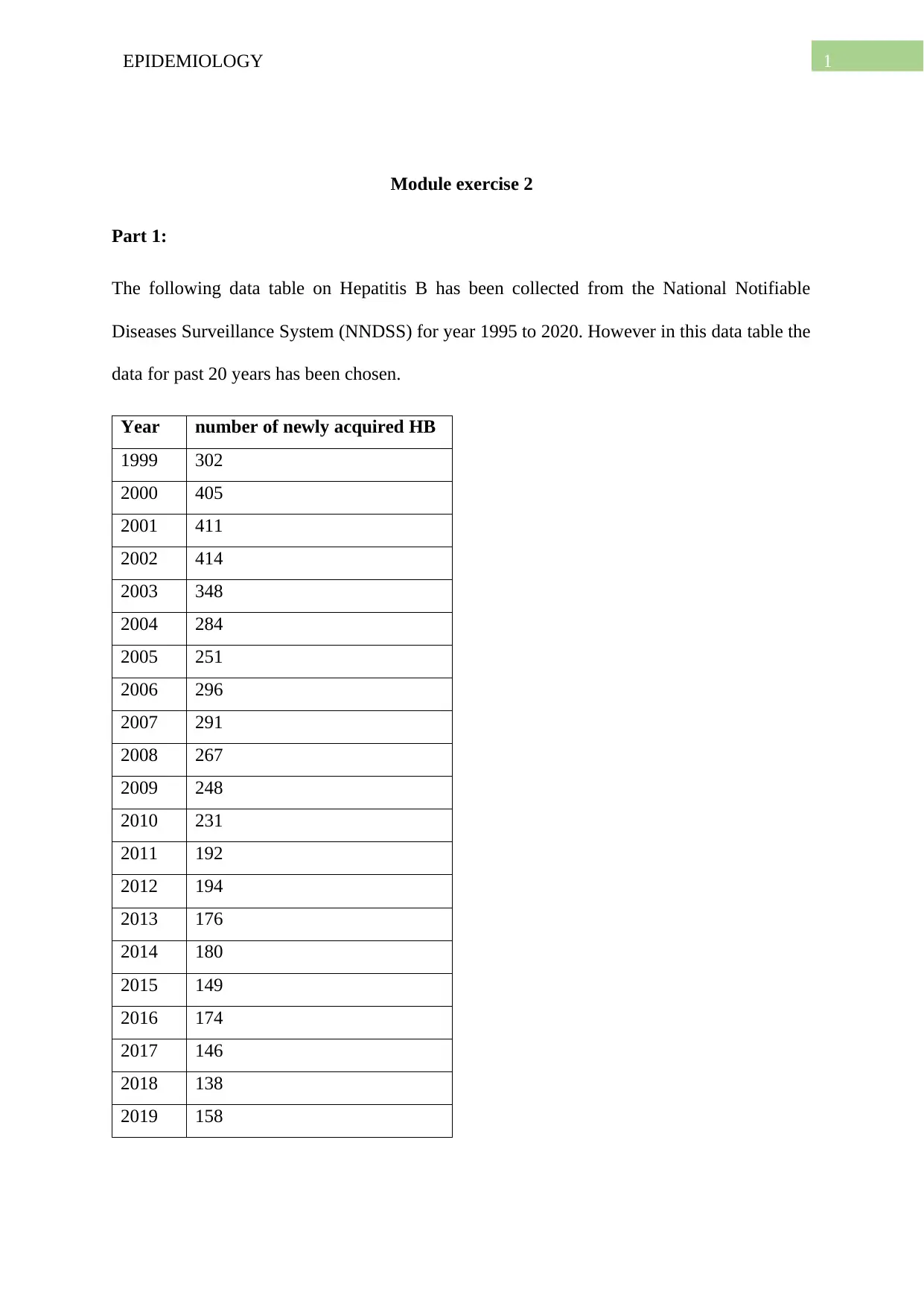
The following data table on Hepatitis B has been collected from the National Notifiable
Diseases Surveillance System (NNDSS) for year 1995 to 2020. However in this data table the
data for past 20 years has been chosen.
Year number of newly acquired HB
1999 302
2000 405
2001 411
2002 414
2003 348
2004 284
2005 251
2006 296
2007 291
2008 267
2009 248
2010 231
2011 192
2012 194
2013 176
2014 180
2015 149
2016 174
2017 146
2018 138
2019 158

2EPIDEMIOLOGY
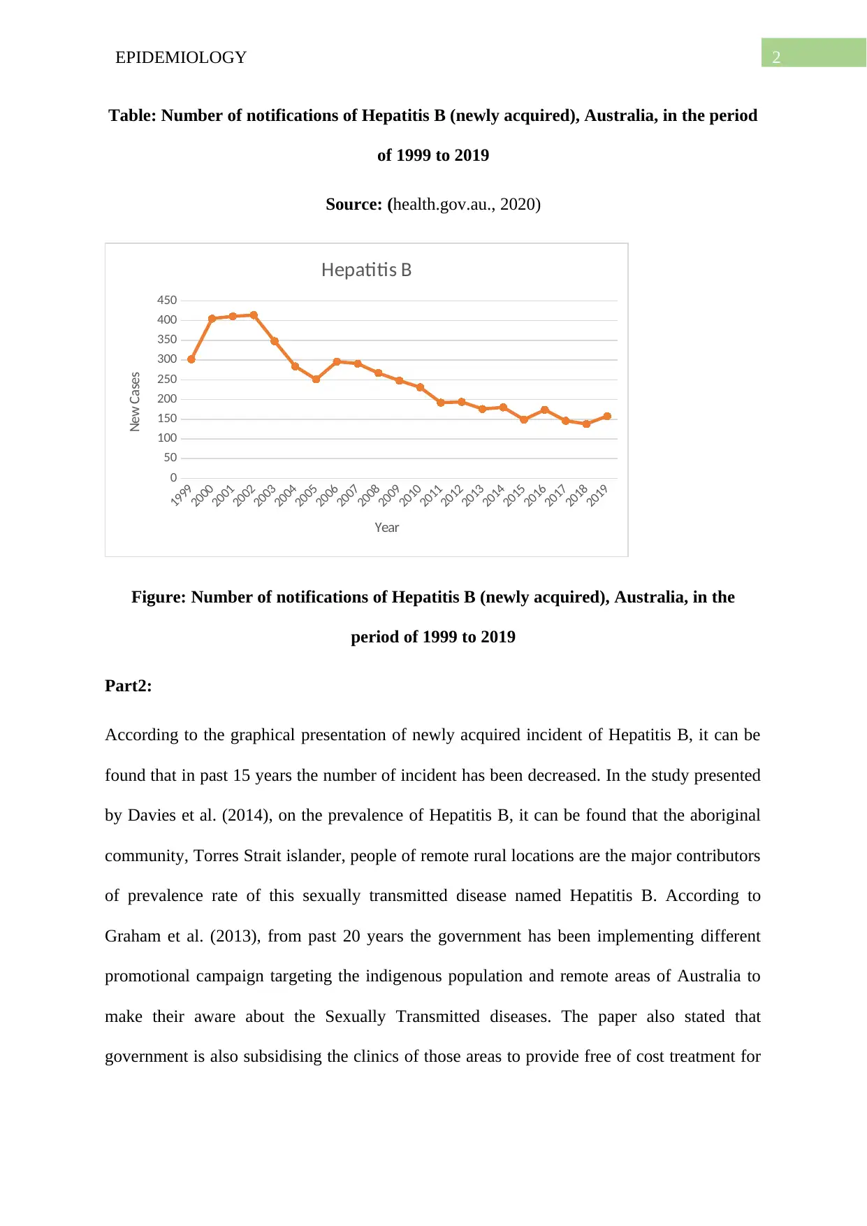
Table: Number of notifications of Hepatitis B (newly acquired), Australia, in the period
of 1999 to 2019
Source: (health.gov.au., 2020)
1999
2000
2001
2002
2003
2004
2005
2006
2007
2008
2009
2010
2011
2012
2013
2014
2015
2016
2017
2018
2019
0
50
100
150
200
250
300
350
400
450
Hepatitis B
Year
New Cases
Figure: Number of notifications of Hepatitis B (newly acquired), Australia, in the
period of 1999 to 2019
Part2:
According to the graphical presentation of newly acquired incident of Hepatitis B, it can be
found that in past 15 years the number of incident has been decreased. In the study presented
by Davies et al. (2014), on the prevalence of Hepatitis B, it can be found that the aboriginal
community, Torres Strait islander, people of remote rural locations are the major contributors
of prevalence rate of this sexually transmitted disease named Hepatitis B. According to
Graham et al. (2013), from past 20 years the government has been implementing different
promotional campaign targeting the indigenous population and remote areas of Australia to
make their aware about the Sexually Transmitted diseases. The paper also stated that
government is also subsidising the clinics of those areas to provide free of cost treatment for

3EPIDEMIOLOGY
hepatitis B. Therefore, it can be major reason behind the declining rate of the incident of
Hepatitis B nationally.
A study on different interventions taken by healthcare organisations with government
association conducted by Silver et al (2015), it can be found that long term screening in rural
areas and remote areas while providing them with healthcare treatment and awareness can
improve the quality of life of the population. Therefore, considering the graphical findings it
can be stated that the current initiations and interventions taken government and primate
healthcare organisations against the sexually transmitted disease named Hepatitis B will
allow them to reduce the prevalence significantly in near future.
Module exercise 3
Part 1:
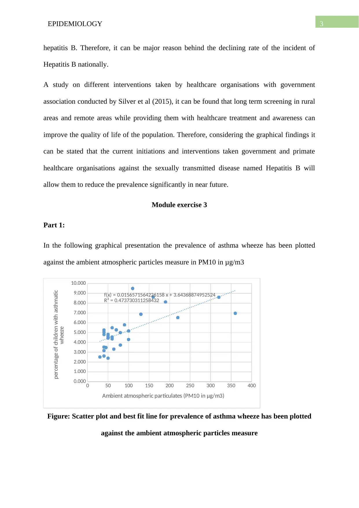
In the following graphical presentation the prevalence of asthma wheeze has been plotted
against the ambient atmospheric particles measure in PM10 in μg/m3
0 50 100 150 200 250 300 350 400
0.000
1.000
2.000
3.000
4.000
5.000
6.000
7.000
8.000
9.000
10.000
f(x) = 0.0156571564226158 x + 3.64368874952524
R² = 0.473730311258432
Ambient atmospheric particulates (PM10 in μg/m3)
percentage of children with asthmatic
wheeze
Figure: Scatter plot and best fit line for prevalence of asthma wheeze has been plotted
against the ambient atmospheric particles measure

4EPIDEMIOLOGY
From the analysis of the computerised liner regression line it can be found that the equation
of the best fit line is y = 0.0157x + 3.6437 and as per the computerised calculation the R2
value is 0.4737. Therefore Pearson coefficient of the correlation r is squire root of R2 .
Hence, Pearson’s Product Moment Correlation Coefficient r= 0.703
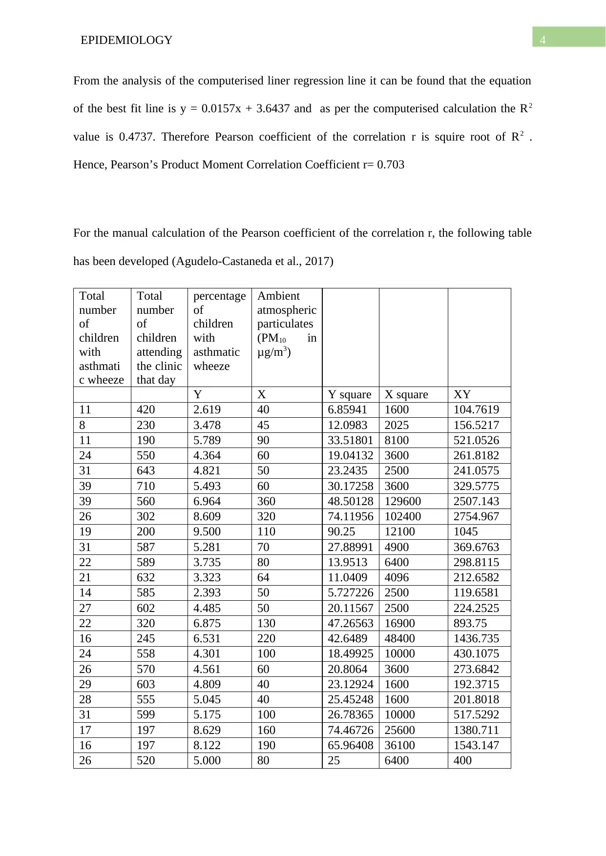
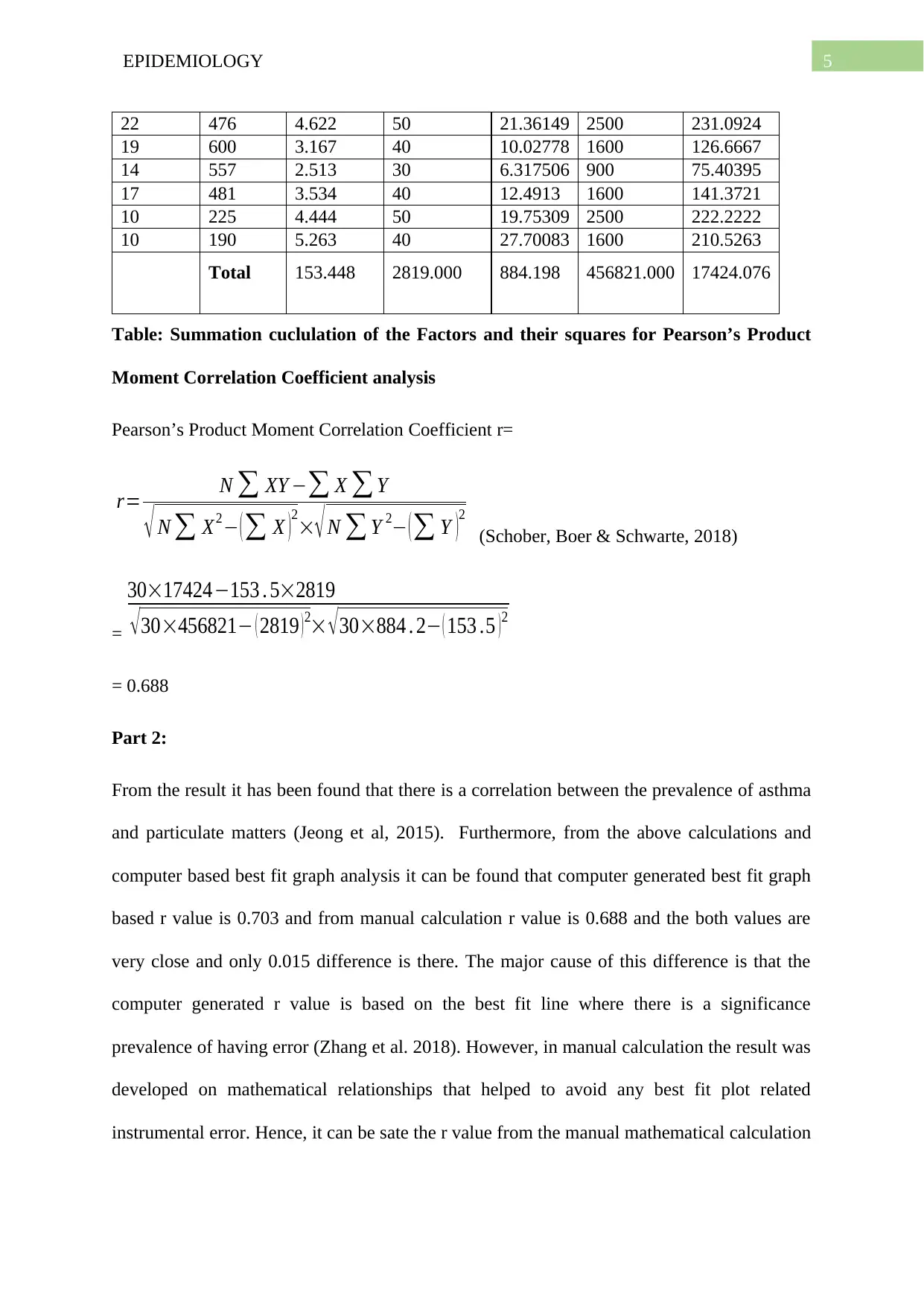
For the manual calculation of the Pearson coefficient of the correlation r, the following table
has been developed (Agudelo-Castaneda et al., 2017)
Total
number
of
children
with
asthmati
c wheeze
Total
number
of
children
attending
the clinic
that day
percentage
of
children
with
asthmatic
wheeze
Ambient
atmospheric
particulates
(PM10 in
μg/m3)
Y X Y square X square XY
11 420 2.619 40 6.85941 1600 104.7619
8 230 3.478 45 12.0983 2025 156.5217
11 190 5.789 90 33.51801 8100 521.0526
24 550 4.364 60 19.04132 3600 261.8182
31 643 4.821 50 23.2435 2500 241.0575
39 710 5.493 60 30.17258 3600 329.5775
39 560 6.964 360 48.50128 129600 2507.143
26 302 8.609 320 74.11956 102400 2754.967
19 200 9.500 110 90.25 12100 1045
31 587 5.281 70 27.88991 4900 369.6763
22 589 3.735 80 13.9513 6400 298.8115
21 632 3.323 64 11.0409 4096 212.6582
14 585 2.393 50 5.727226 2500 119.6581
27 602 4.485 50 20.11567 2500 224.2525
22 320 6.875 130 47.26563 16900 893.75
16 245 6.531 220 42.6489 48400 1436.735
24 558 4.301 100 18.49925 10000 430.1075
26 570 4.561 60 20.8064 3600 273.6842
29 603 4.809 40 23.12924 1600 192.3715
28 555 5.045 40 25.45248 1600 201.8018
31 599 5.175 100 26.78365 10000 517.5292
17 197 8.629 160 74.46726 25600 1380.711
16 197 8.122 190 65.96408 36100 1543.147
26 520 5.000 80 25 6400 400

5EPIDEMIOLOGY
22 476 4.622 50 21.36149 2500 231.0924
19 600 3.167 40 10.02778 1600 126.6667
14 557 2.513 30 6.317506 900 75.40395
17 481 3.534 40 12.4913 1600 141.3721
10 225 4.444 50 19.75309 2500 222.2222
10 190 5.263 40 27.70083 1600 210.5263
Total 153.448 2819.000 884.198 456821.000 17424.076
Table: Summation cuclulation of the Factors and their squares for Pearson’s Product
Moment Correlation Coefficient analysis
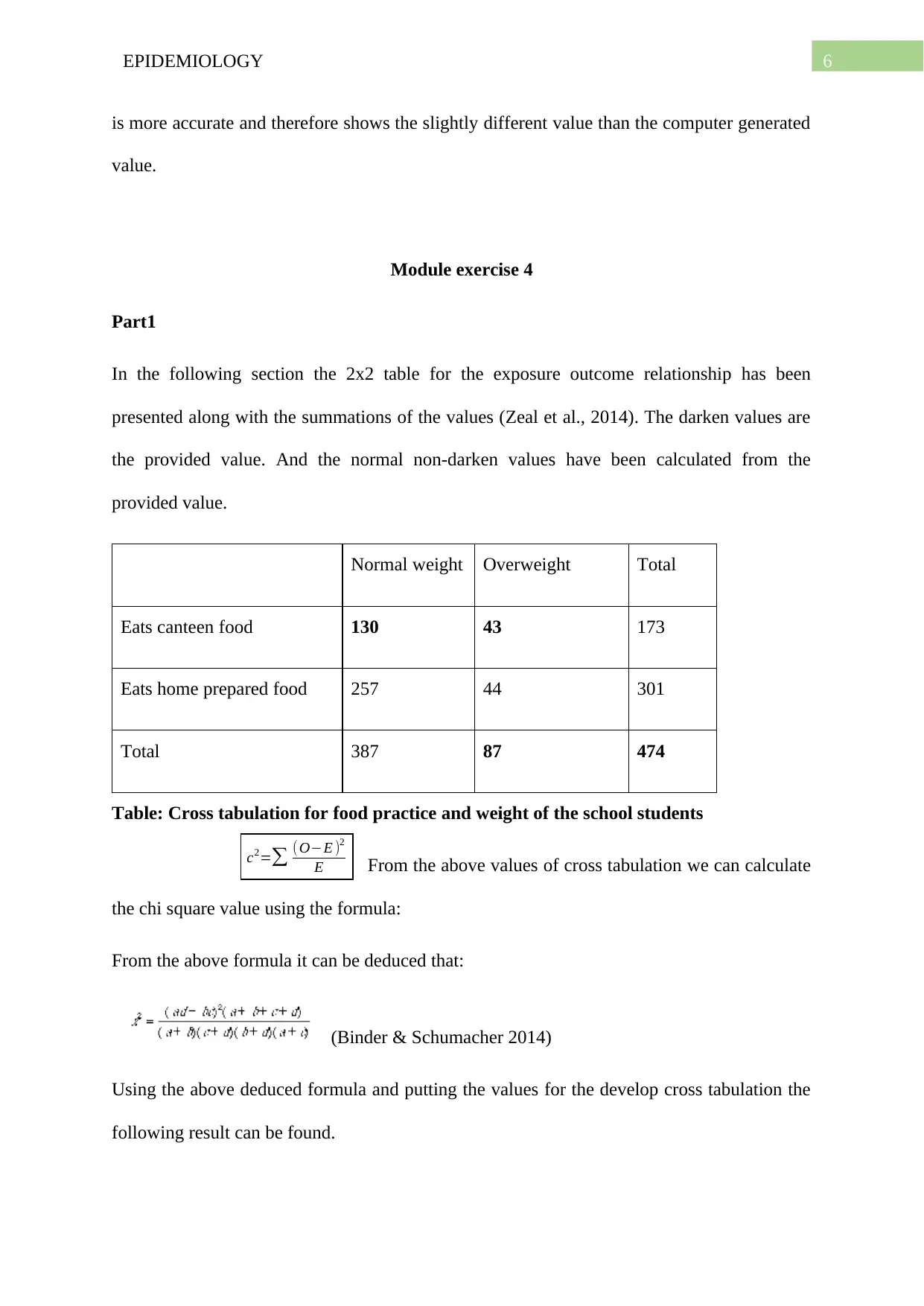
Pearson’s Product Moment Correlation Coefficient r=
r= N ∑ XY −∑ X ∑ Y
√ N ∑ X2− ( ∑ X )
2
× √ N ∑ Y 2− ( ∑ Y )
2
(Schober, Boer & Schwarte, 2018)
=
30×17424−153 . 5×2819
√ 30×456821− ( 2819 ) 2× √ 30×884 . 2− ( 153 .5 ) 2
= 0.688
Part 2:
From the result it has been found that there is a correlation between the prevalence of asthma
and particulate matters (Jeong et al, 2015). Furthermore, from the above calculations and
computer based best fit graph analysis it can be found that computer generated best fit graph
based r value is 0.703 and from manual calculation r value is 0.688 and the both values are
very close and only 0.015 difference is there. The major cause of this difference is that the
computer generated r value is based on the best fit line where there is a significance
prevalence of having error (Zhang et al. 2018). However, in manual calculation the result was
developed on mathematical relationships that helped to avoid any best fit plot related
instrumental error. Hence, it can be sate the r value from the manual mathematical calculation

6EPIDEMIOLOGY
is more accurate and therefore shows the slightly different value than the computer generated
value.
Module exercise 4
Part1
In the following section the 2x2 table for the exposure outcome relationship has been
presented along with the summations of the values (Zeal et al., 2014). The darken values are
the provided value. And the normal non-darken values have been calculated from the
provided value.
Normal weight Overweight Total
Eats canteen food 130 43 173
Eats home prepared food 257 44 301
Total 387 87 474
Table: Cross tabulation for food practice and weight of the school students
From the above values of cross tabulation we can calculate
the chi square value using the formula:
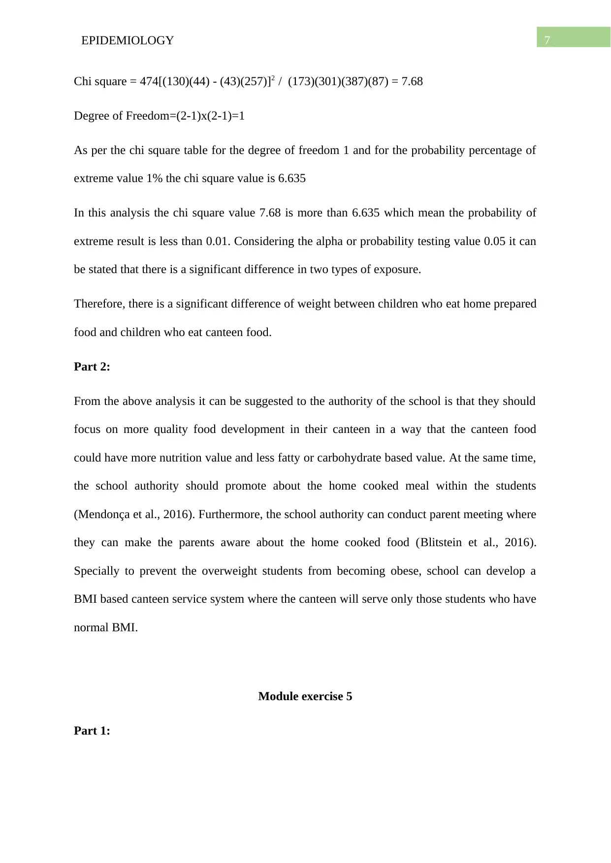
From the above formula it can be deduced that:
(Binder & Schumacher 2014)
Using the above deduced formula and putting the values for the develop cross tabulation the
following result can be found.
c2=∑ (O−E )2
E

7EPIDEMIOLOGY
Chi square = 474[(130)(44) - (43)(257)]2 / (173)(301)(387)(87) = 7.68
Degree of Freedom=(2-1)x(2-1)=1
As per the chi square table for the degree of freedom 1 and for the probability percentage of
extreme value 1% the chi square value is 6.635
In this analysis the chi square value 7.68 is more than 6.635 which mean the probability of
extreme result is less than 0.01. Considering the alpha or probability testing value 0.05 it can
be stated that there is a significant difference in two types of exposure.
Therefore, there is a significant difference of weight between children who eat home prepared
food and children who eat canteen food.
Part 2:
From the above analysis it can be suggested to the authority of the school is that they should
focus on more quality food development in their canteen in a way that the canteen food
could have more nutrition value and less fatty or carbohydrate based value. At the same time,
the school authority should promote about the home cooked meal within the students
(Mendonça et al., 2016). Furthermore, the school authority can conduct parent meeting where
they can make the parents aware about the home cooked food (Blitstein et al., 2016).
Specially to prevent the overweight students from becoming obese, school can develop a
BMI based canteen service system where the canteen will serve only those students who have
normal BMI.
Module exercise 5
Part 1:

8EPIDEMIOLOGY
In order carry out the relative risk analysis the following cross tabulation table has been
developed to present the various exposure and outcomes based values as well as their
summations.
Food eaten Bankers ill Bankers not ill Total Cumulative
Incidence
(CI)
Cream of
mushroom soup
83 30 113 0.735
Shrimp cocktail 44 36 80 0.550
Chicken a la
king
74 34 108 0.685
Vegetarian
platter
13 46 59 0.220
Ice cream with
choc sauce
38 32 70 0.543
Coffee 11 42 53 0.208
Table: cumulative incident calculations for all type of food eaten
Based on the above cumulative incident values the relative risks of the all corresponding
combinations of the exposure has been calculated and presented in the following section. In
order to calculate the relative risk the following formula has been used:
Relative risk = (cumulative risk in exposed population/cumulative risk in un-exposed
population)
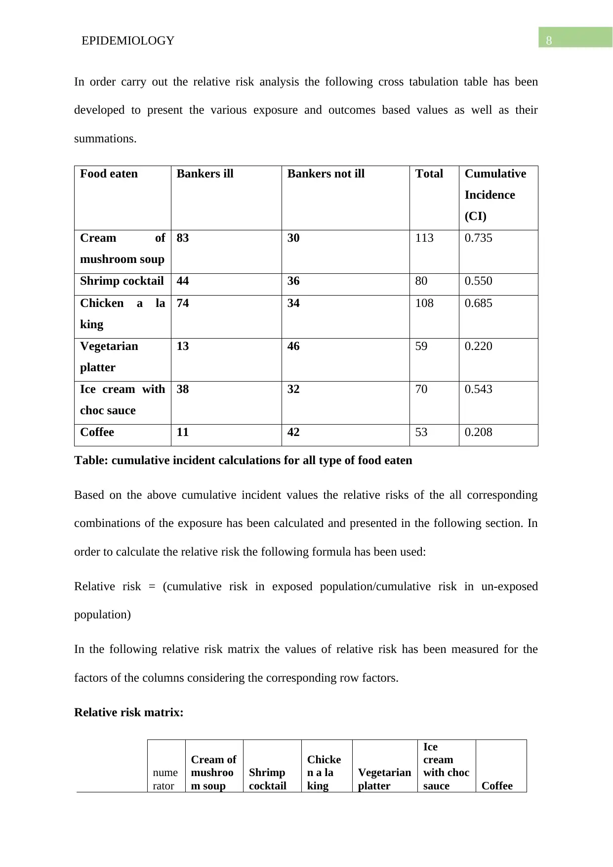
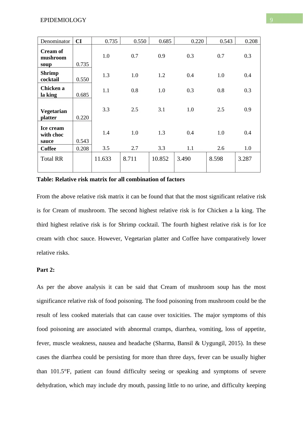
In the following relative risk matrix the values of relative risk has been measured for the
factors of the columns considering the corresponding row factors.
Relative risk matrix:
nume
rator
Cream of
mushroo
m soup
Shrimp
cocktail
Chicke
n a la
king
Vegetarian
platter
Ice
cream
with choc
sauce Coffee

9EPIDEMIOLOGY
Denominator CI 0.735 0.550 0.685 0.220 0.543 0.208
Cream of
mushroom
soup 0.735
1.0 0.7 0.9 0.3 0.7 0.3
Shrimp
cocktail 0.550 1.3 1.0 1.2 0.4 1.0 0.4
Chicken a
la king 0.685 1.1 0.8 1.0 0.3 0.8 0.3
Vegetarian
platter 0.220
3.3 2.5 3.1 1.0 2.5 0.9
Ice cream
with choc
sauce 0.543
1.4 1.0 1.3 0.4 1.0 0.4
Coffee 0.208 3.5 2.7 3.3 1.1 2.6 1.0
Total RR 11.633 8.711 10.852 3.490 8.598 3.287
Table: Relative risk matrix for all combination of factors
From the above relative risk matrix it can be found that that the most significant relative risk
is for Cream of mushroom. The second highest relative risk is for Chicken a la king. The
third highest relative risk is for Shrimp cocktail. The fourth highest relative risk is for Ice
cream with choc sauce. However, Vegetarian platter and Coffee have comparatively lower
relative risks.
Part 2:
As per the above analysis it can be said that Cream of mushroom soup has the most
significance relative risk of food poisoning. The food poisoning from mushroom could be the
result of less cooked materials that can cause over toxicities. The major symptoms of this
food poisoning are associated with abnormal cramps, diarrhea, vomiting, loss of appetite,
fever, muscle weakness, nausea and headache (Sharma, Bansil & Uygungil, 2015). In these
cases the diarrhea could be persisting for more than three days, fever can be usually higher
than 101.5°F, patient can found difficulty seeing or speaking and symptoms of severe
dehydration, which may include dry mouth, passing little to no urine, and difficulty keeping

10EPIDEMIOLOGY
fluids down (Dutta, Kalita & Pegu, 2013). However, in case of food poisoning from protein
based food such as Chicken a la king patient can have the above symptoms as well as the visible
blood in urine. Therefore, in such cases immediate consultation with medical professionals will be
highly required (Kunwar et al., 2013).
Module exercise 6
Part 1:
The questions for the chosen pattern of badly designed interview questions are:
 Leading question: Do you face severe stress symptoms because of aircraft noise?
 Threatening question: Knowing the fact that no one can be blamed for the noise, do
you still want to hold your complains about noise level?
 Ambiguous question: Rate your issues you have faced due to noise level?
 Insensitive question: How much anger do you show to your family member because
of being irritated from the aircraft noise?
 Unreasonable question: Do your any relative or friend have any anxiety issues
because of noise?
 Unstandardised question: How much stress symptoms do you have?
Part2:
Considering the reliability, validity, specificity and other authenticity measures the above
poorly developed interview questions have been redeveloped (Castillo-Montoya, 2016). After
rewriting the following questions have been developed:
Q1. Have you ever experience any stress issues such as agitation or anxiety or tiredness due
to prolonged hours of aircraft sound?

11EPIDEMIOLOGY
Q2. Do you think that any noise reduction initiation could be taken about this fact to reduce
the noise level? (Brown et al., 2013)
Q3. How frequent do you experience stress symptoms such as agitation or anxiety or
tiredness due to prolonged hours of aircraft sound? (Mann, 2016)
Q4. Have you ever lost your temper because of the agitating aircraft noise?
Q5. Have you ever experienced sleeping disturbance because aircraft noise?
For question six, the questionnaire criteria are the subject which is consulting to therapist, the
specific question that is the frequency of constancy, the reason which is the stress related
issue, the measurable condition is the frequency (Jamshed, 2014). Therefore the question six
will be:
Q6. Have you ever or how frequently have consulted to a therapist regarding any stress
related issues?
Module exercise 7:
Part 1:
Total population in rural town is 2000
EHO believes that the occupants of about one-half of the houses might have a borehole water
supply in addition to the treated Council supply (Byrne,, Anda & Ho, 2019). Therefore, the
effect size is one –half or 50%
Therefore expected prevalence P1= 50%= 0.5