Statistical Methods in Epidemiology (401176) Assignment 1 - WSU 2017

This assignment solution from Western Sydney University's School of Medicine covers statistical methods in epidemiology. It addresses descriptive statistics, confounding, effect modification, and various statistical tests. The assignment includes questions on graphical methods, comparing weight gain with different diets, and the use of statistical measures for variables with different measurement scales. It further explores confounding and effect modification, consequences of not adjusting for confounding, and the limitations of stratification. Questions involve the application of the Mantel-Haenszel and Woolf estimators, the Breslow and Day test, and hypothesis testing related to relative odds and confidence intervals. The assignment requires interpreting results, drawing conclusions, and performing analyses on case-control studies and birthweight data, with a focus on the impact of smoking and other variables. The student is expected to use SAS codes, scientific calculators, and Microsoft Excel to analyze the provided data and answer the questions effectively. The assignment is designed to assess the student's understanding of epidemiological concepts and their ability to apply statistical methods to analyze and interpret data. The student also needs to comment on the difference in the results of the two analyses.

1
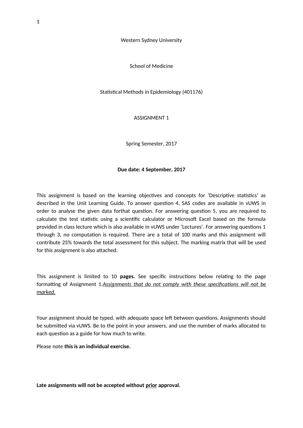
Western Sydney University
School of Medicine
Statistical Methods in Epidemiology (401176)
ASSIGNMENT 1
Spring Semester, 2017
Due date: 4 September, 2017
This assignment is based on the learning objectives and concepts for ‘Descriptive statistics’ as
described in the Unit Learning Guide. To answer question 4, SAS codes are available in vUWS in
order to analyse the given data forthat question. For answering question 5, you are required to
calculate the test statistic using a scientific calculator or Microsoft Excel based on the formula
provided in class lecture which is also available in vUWS under ‘Lectures’. For answering questions 1
through 3, no computation is required. There are a total of 100 marks and this assignment will
contribute 25% towards the total assessment for this subject. The marking matrix that will be used
for this assignment is also attached.
This assignment is limited to 10 pages. See specific instructions below relating to the page
formatting of Assignment 1.Assignments that do not comply with these specifications will not be
marked.
Your assignment should be typed, with adequate space left between questions. Assignments should
be submitted via vUWS. Be to the point in your answers, and use the number of marks allocated to
each question as a guide for how much to write.
Please note this is an individual exercise.
Late assignments will not be accepted without prior approval.

2
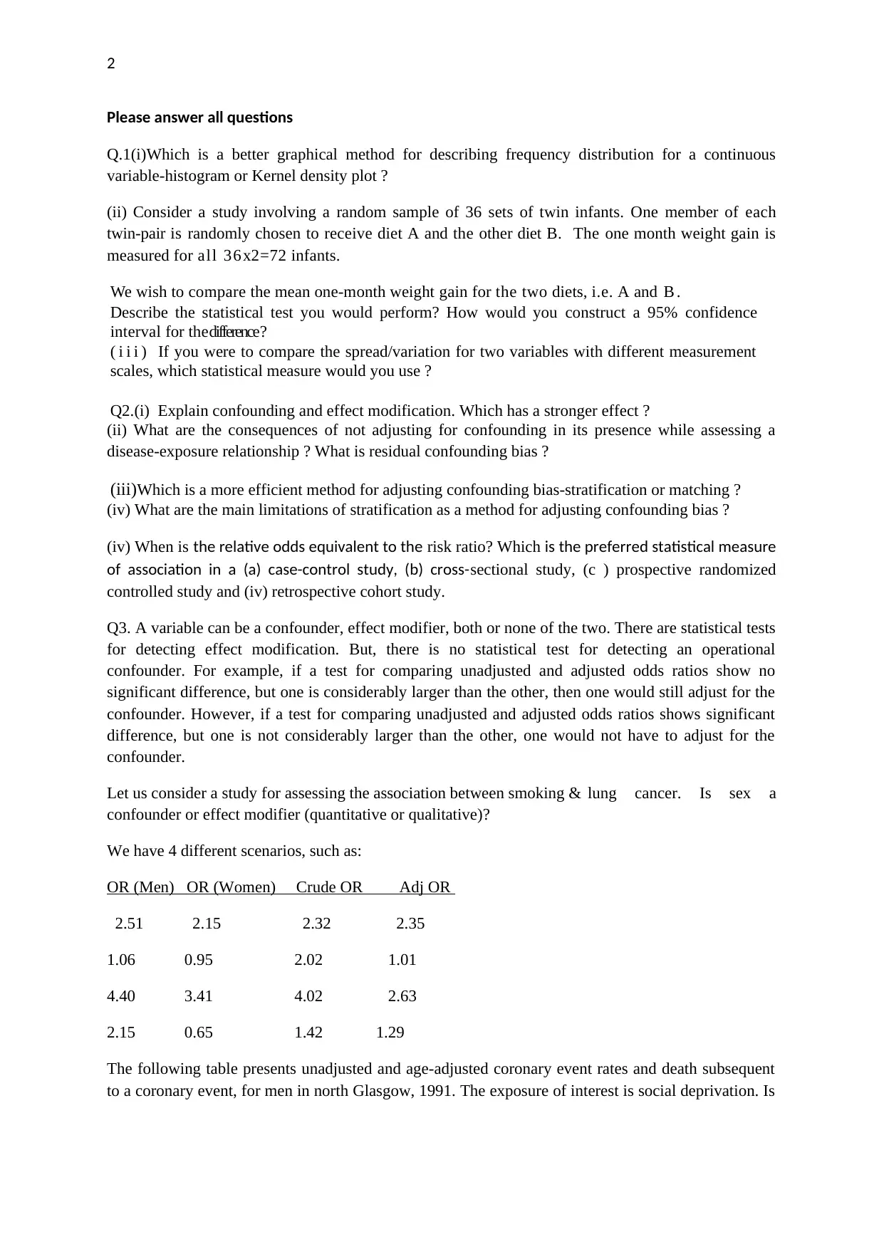
Please answer all questions
Q.1(i)Which is a better graphical method for describing frequency distribution for a continuous
variable-histogram or Kernel density plot ?
(ii) Consider a study involving a random sample of 36 sets of twin infants. One member of each
twin-pair is randomly chosen to receive diet A and the other diet B. The one month weight gain is
measured for all 36x2=72 infants.
We wish to compare the mean one-month weight gain for the two diets, i.e. A and B .
Describe the statistical test you would perform? How would you construct a 95% confidence
interval for the difference?
( i i i ) If you were to compare the spread/variation for two variables with different measurement
scales, which statistical measure would you use ?
Q2.(i) Explain confounding and effect modification. Which has a stronger effect ?
(ii) What are the consequences of not adjusting for confounding in its presence while assessing a
disease-exposure relationship ? What is residual confounding bias ?
(iii)Which is a more efficient method for adjusting confounding bias-stratification or matching ?
(iv) What are the main limitations of stratification as a method for adjusting confounding bias ?
(iv) When is the relative odds equivalent to the risk ratio? Which is the preferred statistical measure
of association in a (a) case-control study, (b) cross-sectional study, (c ) prospective randomized
controlled study and (iv) retrospective cohort study.
Q3. A variable can be a confounder, effect modifier, both or none of the two. There are statistical tests
for detecting effect modification. But, there is no statistical test for detecting an operational
confounder. For example, if a test for comparing unadjusted and adjusted odds ratios show no
significant difference, but one is considerably larger than the other, then one would still adjust for the
confounder. However, if a test for comparing unadjusted and adjusted odds ratios shows significant
difference, but one is not considerably larger than the other, one would not have to adjust for the
confounder.
Let us consider a study for assessing the association between smoking & lung cancer. Is sex a
confounder or effect modifier (quantitative or qualitative)?
We have 4 different scenarios, such as:
OR (Men) OR (Women) Crude OR Adj OR
2.51 2.15 2.32 2.35
1.06 0.95 2.02 1.01
4.40 3.41 4.02 2.63
2.15 0.65 1.42 1.29
The following table presents unadjusted and age-adjusted coronary event rates and death subsequent
to a coronary event, for men in north Glasgow, 1991. The exposure of interest is social deprivation. Is

3
age a confounder in the relationship between social deprivation and coronary event rate and coronary
death?
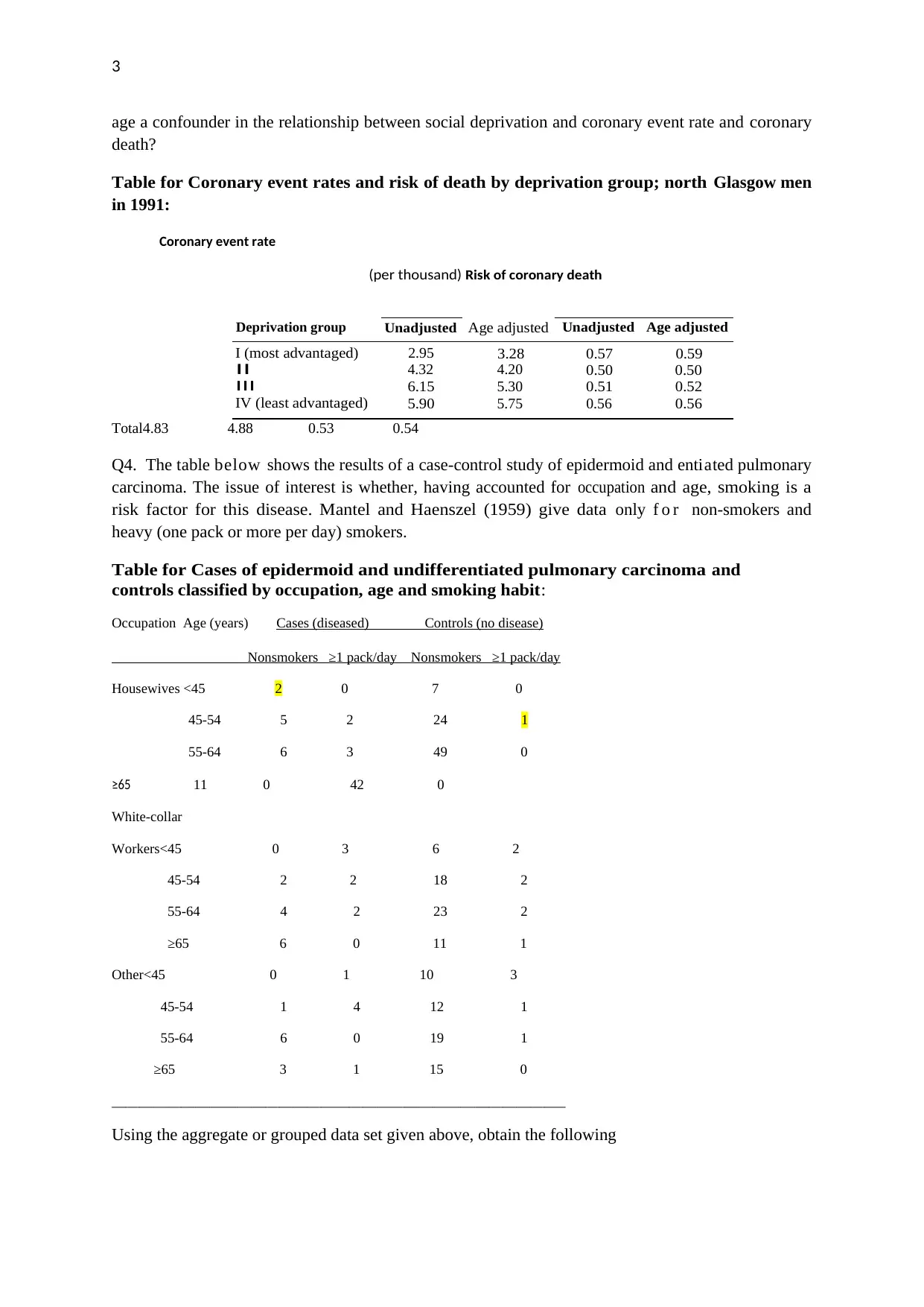
Table for Coronary event rates and risk of death by deprivation group; north Glasgow men
in 1991:
Coronary event rate
(per thousand) Risk of coronary death
Deprivation group Unadjusted Age adjusted Unadjusted Age adjusted
I (most advantaged) 2.95 3.28 0.57 0.59
II 4.32 4.20 0.50 0.50
III 6.15 5.30 0.51 0.52
IV (least advantaged) 5.90 5.75 0.56 0.56
Total4.83 4.88 0.53 0.54
Q4. The table below shows the results of a case-control study of epidermoid and entiated pulmonary
carcinoma. The issue of interest is whether, having accounted for occupation and age, smoking is a
risk factor for this disease. Mantel and Haenszel (1959) give data only f o r non-smokers and
heavy (one pack or more per day) smokers.
Table for Cases of epidermoid and undifferentiated pulmonary carcinoma and
controls classified by occupation, age and smoking habit:
Occupation Age (years) Cases (diseased) Controls (no disease)
Nonsmokers ≥1 pack/day Nonsmokers ≥1 pack/day
Housewives <45 2 0 7 0
45-54 5 2 24 1
55-64 6 3 49 0
≥65 11 0 42 0
White-collar
Workers<45 0 3 6 2
45-54 2 2 18 2
55-64 4 2 23 2
≥65 6 0 11 1
Other<45 0 1 10 3
45-54 1 4 12 1
55-64 6 0 19 1
≥65 3 1 15 0
_________________________________________________________________
Using the aggregate or grouped data set given above, obtain the following

4
(i) Interpret Breslow and Day test for homogeneity of relative odds across the strata. Are the
relative odds homogeneous across the strata ?
(ii) If the relative odds are the same across the strata, interpret the Mantel-Haenszel test on
whether the common relative odds differs significantly from 1. Is there a significant
association between smoking and pulmonary epidermoid and entiated carcinoma ?
(iii) Interpret the Mantel-Haenszel and Woolf (logit) estimators of common relative odds and
the corresponding 95% confidence intervals.
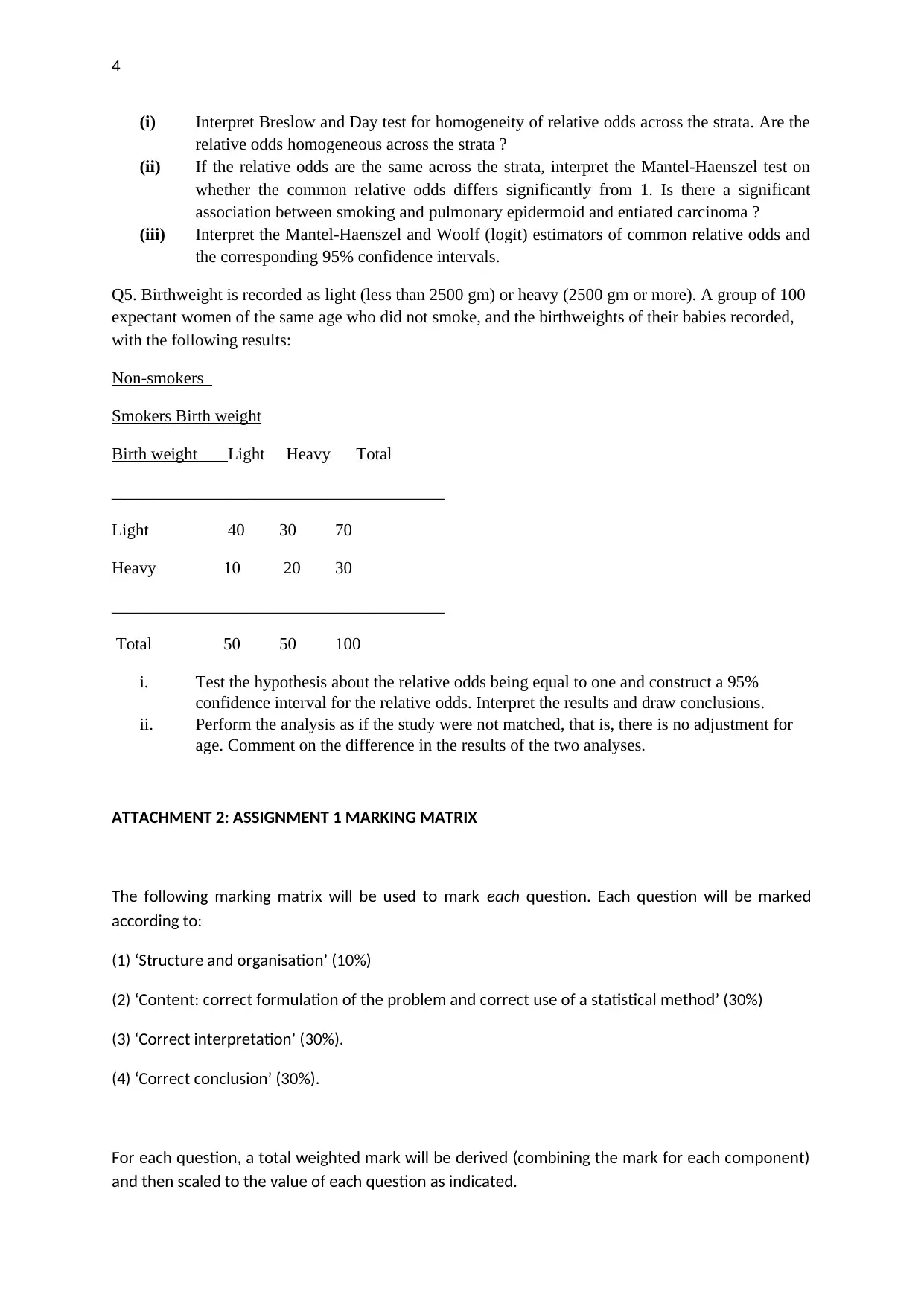
Q5. Birthweight is recorded as light (less than 2500 gm) or heavy (2500 gm or more). A group of 100
expectant women of the same age who did not smoke, and the birthweights of their babies recorded,
with the following results:
Non-smokers
Smokers Birth weight
Birth weight Light Heavy Total
_______________________________________
Light 40 30 70
Heavy 10 20 30
_______________________________________
Total 50 50 100
i. Test the hypothesis about the relative odds being equal to one and construct a 95%
confidence interval for the relative odds. Interpret the results and draw conclusions.
ii. Perform the analysis as if the study were not matched, that is, there is no adjustment for
age. Comment on the difference in the results of the two analyses.
ATTACHMENT 2: ASSIGNMENT 1 MARKING MATRIX
The following marking matrix will be used to mark each question. Each question will be marked
according to:
(1) ‘Structure and organisation’ (10%)
(2) ‘Content: correct formulation of the problem and correct use of a statistical method’ (30%)
(3) ‘Correct interpretation’ (30%).
(4) ‘Correct conclusion’ (30%).
For each question, a total weighted mark will be derived (combining the mark for each component)
and then scaled to the value of each question as indicated.