Derivatives Trading and Hedging Project: FR2211 Coursework Analysis
VerifiedAdded on 2023/04/21
|26
|4972
|402
Project
AI Summary
This project analyzes derivatives trading and hedging strategies for equity portfolios using real-world data. The student utilized R programming to address questions related to excess daily returns, mean and standard deviation calculations, and estimating alpha, beta, t-statistics, and R-squared values for software and gold portfolios. The project explores the Capital Asset Pricing Model (CAPM) to assess portfolio performance, determine optimal hedging strategies using S&P 500 and Nasdaq 100 mini futures contracts, and calculate cumulative gains. The analysis includes plotting index levels and spot-futures bases, interpreting graphs, and evaluating the value of hedged portfolio positions across different time periods. Furthermore, the project examines the relationship between daily excess returns and the risk-free rate, compares CAPM results for unhedged and hedged scenarios, and provides interpretations and conclusions based on the findings. The solution demonstrates an understanding of financial derivatives and risk management techniques.

DERIVATIVES
1
STATISTICS
DERIVATIVES
Student Name:
Name of Institution:
1
STATISTICS
DERIVATIVES
Student Name:
Name of Institution:
Paraphrase This Document
Need a fresh take? Get an instant paraphrase of this document with our AI Paraphraser
2
> #Importing the dataset
> Data_set<-read.csv("F:/Data.csv")
> #Question 1:
> #Excess daily returns has been calculated by getting the difference between the returns and the
risk- free interest rate.The risk- free rate has been taken to be 2% (0.02). The caluculations have
been done in excel. The values of excess daily returns can be extracted from data set using the
code below.
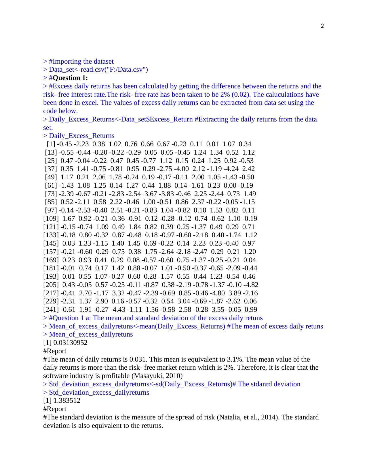
> Daily_Excess_Returns<-Data_set$Excess_Return #Extracting the daily returns from the data
set.
> Daily_Excess_Returns
[1] -0.45 -2.23 0.38 1.02 0.76 0.66 0.67 -0.23 0.11 0.01 1.07 0.34
[13] -0.55 -0.44 -0.20 -0.22 -0.29 0.05 0.05 -0.45 1.24 1.34 0.52 1.12
[25] 0.47 -0.04 -0.22 0.47 0.45 -0.77 1.12 0.15 0.24 1.25 0.92 -0.53
[37] 0.35 1.41 -0.75 -0.81 0.95 0.29 -2.75 -4.00 2.12 -1.19 -4.24 2.42
[49] 1.17 0.21 2.06 1.78 -0.24 0.19 -0.17 -0.11 2.00 1.05 -1.43 -0.50
[61] -1.43 1.08 1.25 0.14 1.27 0.44 1.88 0.14 -1.61 0.23 0.00 -0.19
[73] -2.39 -0.67 -0.21 -2.83 -2.54 3.67 -3.83 -0.46 2.25 -2.44 0.73 1.49
[85] 0.52 -2.11 0.58 2.22 -0.46 1.00 -0.51 0.86 2.37 -0.22 -0.05 -1.15
[97] -0.14 -2.53 -0.40 2.51 -0.21 -0.83 1.04 -0.82 0.10 1.53 0.82 0.11
[109] 1.67 0.92 -0.21 -0.36 -0.91 0.12 -0.28 -0.12 0.74 -0.62 1.10 -0.19
[121] -0.15 -0.74 1.09 0.49 1.84 0.82 0.39 0.25 -1.37 0.49 0.29 0.71
[133] -0.18 0.80 -0.32 0.87 -0.48 0.18 -0.97 -0.60 -2.18 0.40 -1.74 1.12
[145] 0.03 1.33 -1.15 1.40 1.45 0.69 -0.22 0.14 2.23 0.23 -0.40 0.97
[157] -0.21 -0.60 0.29 0.75 0.38 1.75 -2.64 -2.18 -2.47 0.29 0.21 1.20
[169] 0.23 0.93 0.41 0.29 0.08 -0.57 -0.60 0.75 -1.37 -0.25 -0.21 0.04
[181] -0.01 0.74 0.17 1.42 0.88 -0.07 1.01 -0.50 -0.37 -0.65 -2.09 -0.44
[193] 0.01 0.55 1.07 -0.27 0.60 0.28 -1.57 0.55 -0.44 1.23 -0.54 0.46
[205] 0.43 -0.05 0.57 -0.25 -0.11 -0.87 0.38 -2.19 -0.78 -1.37 -0.10 -4.82
[217] -0.41 2.70 -1.17 3.32 -0.47 -2.39 -0.69 0.85 -0.46 -4.80 3.89 -2.16
[229] -2.31 1.37 2.90 0.16 -0.57 -0.32 0.54 3.04 -0.69 -1.87 -2.62 0.06
[241] -0.61 1.91 -0.27 -4.43 -1.11 1.56 -0.58 2.58 -0.28 3.55 -0.05 0.99
> #Question 1 a: The mean and standard deviation of the excess daily retuns
> Mean_of_excess_dailyretuns<-mean(Daily_Excess_Returns) #The mean of excess daily retuns
> Mean_of_excess_dailyretuns
[1] 0.03130952
#Report
#The mean of daily returns is 0.031. This mean is equivalent to 3.1%. The mean value of the
daily returns is more than the risk- free market return which is 2%. Therefore, it is clear that the
software industry is profitable (Masayuki, 2010)
> Std_deviation_excess_dailyreturns<-sd(Daily_Excess_Returns)# The stdanrd deviation
> Std_deviation_excess_dailyreturns
[1] 1.383512
#Report
#The standard deviation is the measure of the spread of risk (Natalia, et al., 2014). The standard
deviation is also equivalent to the returns.
> #Importing the dataset
> Data_set<-read.csv("F:/Data.csv")
> #Question 1:
> #Excess daily returns has been calculated by getting the difference between the returns and the
risk- free interest rate.The risk- free rate has been taken to be 2% (0.02). The caluculations have
been done in excel. The values of excess daily returns can be extracted from data set using the
code below.
> Daily_Excess_Returns<-Data_set$Excess_Return #Extracting the daily returns from the data
set.
> Daily_Excess_Returns
[1] -0.45 -2.23 0.38 1.02 0.76 0.66 0.67 -0.23 0.11 0.01 1.07 0.34
[13] -0.55 -0.44 -0.20 -0.22 -0.29 0.05 0.05 -0.45 1.24 1.34 0.52 1.12
[25] 0.47 -0.04 -0.22 0.47 0.45 -0.77 1.12 0.15 0.24 1.25 0.92 -0.53
[37] 0.35 1.41 -0.75 -0.81 0.95 0.29 -2.75 -4.00 2.12 -1.19 -4.24 2.42
[49] 1.17 0.21 2.06 1.78 -0.24 0.19 -0.17 -0.11 2.00 1.05 -1.43 -0.50
[61] -1.43 1.08 1.25 0.14 1.27 0.44 1.88 0.14 -1.61 0.23 0.00 -0.19
[73] -2.39 -0.67 -0.21 -2.83 -2.54 3.67 -3.83 -0.46 2.25 -2.44 0.73 1.49
[85] 0.52 -2.11 0.58 2.22 -0.46 1.00 -0.51 0.86 2.37 -0.22 -0.05 -1.15
[97] -0.14 -2.53 -0.40 2.51 -0.21 -0.83 1.04 -0.82 0.10 1.53 0.82 0.11
[109] 1.67 0.92 -0.21 -0.36 -0.91 0.12 -0.28 -0.12 0.74 -0.62 1.10 -0.19
[121] -0.15 -0.74 1.09 0.49 1.84 0.82 0.39 0.25 -1.37 0.49 0.29 0.71
[133] -0.18 0.80 -0.32 0.87 -0.48 0.18 -0.97 -0.60 -2.18 0.40 -1.74 1.12
[145] 0.03 1.33 -1.15 1.40 1.45 0.69 -0.22 0.14 2.23 0.23 -0.40 0.97
[157] -0.21 -0.60 0.29 0.75 0.38 1.75 -2.64 -2.18 -2.47 0.29 0.21 1.20
[169] 0.23 0.93 0.41 0.29 0.08 -0.57 -0.60 0.75 -1.37 -0.25 -0.21 0.04
[181] -0.01 0.74 0.17 1.42 0.88 -0.07 1.01 -0.50 -0.37 -0.65 -2.09 -0.44
[193] 0.01 0.55 1.07 -0.27 0.60 0.28 -1.57 0.55 -0.44 1.23 -0.54 0.46
[205] 0.43 -0.05 0.57 -0.25 -0.11 -0.87 0.38 -2.19 -0.78 -1.37 -0.10 -4.82
[217] -0.41 2.70 -1.17 3.32 -0.47 -2.39 -0.69 0.85 -0.46 -4.80 3.89 -2.16
[229] -2.31 1.37 2.90 0.16 -0.57 -0.32 0.54 3.04 -0.69 -1.87 -2.62 0.06
[241] -0.61 1.91 -0.27 -4.43 -1.11 1.56 -0.58 2.58 -0.28 3.55 -0.05 0.99
> #Question 1 a: The mean and standard deviation of the excess daily retuns
> Mean_of_excess_dailyretuns<-mean(Daily_Excess_Returns) #The mean of excess daily retuns
> Mean_of_excess_dailyretuns
[1] 0.03130952
#Report
#The mean of daily returns is 0.031. This mean is equivalent to 3.1%. The mean value of the
daily returns is more than the risk- free market return which is 2%. Therefore, it is clear that the
software industry is profitable (Masayuki, 2010)
> Std_deviation_excess_dailyreturns<-sd(Daily_Excess_Returns)# The stdanrd deviation
> Std_deviation_excess_dailyreturns
[1] 1.383512
#Report
#The standard deviation is the measure of the spread of risk (Natalia, et al., 2014). The standard
deviation is also equivalent to the returns.
3
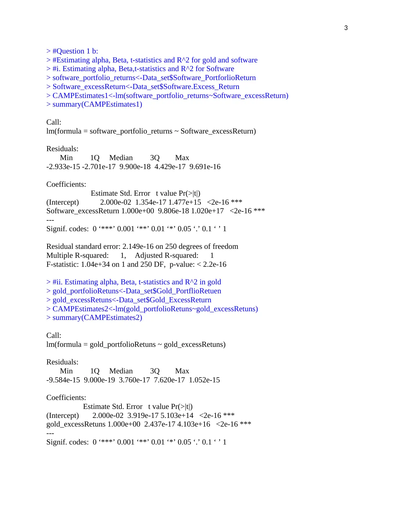
> #Question 1 b:
> #Estimating alpha, Beta, t-statistics and R^2 for gold and software
> #i. Estimating alpha, Beta,t-statistics and R^2 for Software
> software_portfolio_returns<-Data_set$Software_PortforlioReturn
> Software_excessReturn<-Data_set$Software.Excess_Return
> CAMPEstimates1<-lm(software_portfolio_returns~Software_excessReturn)
> summary(CAMPEstimates1)
Call:
lm(formula = software_portfolio_returns ~ Software_excessReturn)
Residuals:
Min 1Q Median 3Q Max
-2.933e-15 -2.701e-17 9.900e-18 4.429e-17 9.691e-16
Coefficients:
Estimate Std. Error t value Pr(>|t|)
(Intercept) 2.000e-02 1.354e-17 1.477e+15 <2e-16 ***
Software_excessReturn 1.000e+00 9.806e-18 1.020e+17 <2e-16 ***
---
Signif. codes: 0 ‘***’ 0.001 ‘**’ 0.01 ‘*’ 0.05 ‘.’ 0.1 ‘ ’ 1
Residual standard error: 2.149e-16 on 250 degrees of freedom
Multiple R-squared: 1, Adjusted R-squared: 1
F-statistic: 1.04e+34 on 1 and 250 DF, p-value: < 2.2e-16
> #ii. Estimating alpha, Beta, t-statistics and R^2 in gold
> gold_portfolioRetuns<-Data_set$Gold_PortflioRetuen
> gold_excessRetuns<-Data_set$Gold_ExcessReturn
> CAMPEstimates2<-lm(gold_portfolioRetuns~gold_excessRetuns)
> summary(CAMPEstimates2)
Call:
lm(formula = gold_portfolioRetuns ~ gold_excessRetuns)
Residuals:
Min 1Q Median 3Q Max
-9.584e-15 9.000e-19 3.760e-17 7.620e-17 1.052e-15
Coefficients:
Estimate Std. Error t value Pr(>|t|)
(Intercept) 2.000e-02 3.919e-17 5.103e+14 <2e-16 ***
gold_excessRetuns 1.000e+00 2.437e-17 4.103e+16 <2e-16 ***
---
Signif. codes: 0 ‘***’ 0.001 ‘**’ 0.01 ‘*’ 0.05 ‘.’ 0.1 ‘ ’ 1
⊘ This is a preview!⊘
Do you want full access?
Subscribe today to unlock all pages.
Trusted by 1+ million students worldwide
4
Residual standard error: 6.215e-16 on 250 degrees of freedom
Multiple R-squared: 1, Adjusted R-squared: 1
F-statistic: 1.684e+33 on 1 and 250 DF, p-value: < 2.2e-16
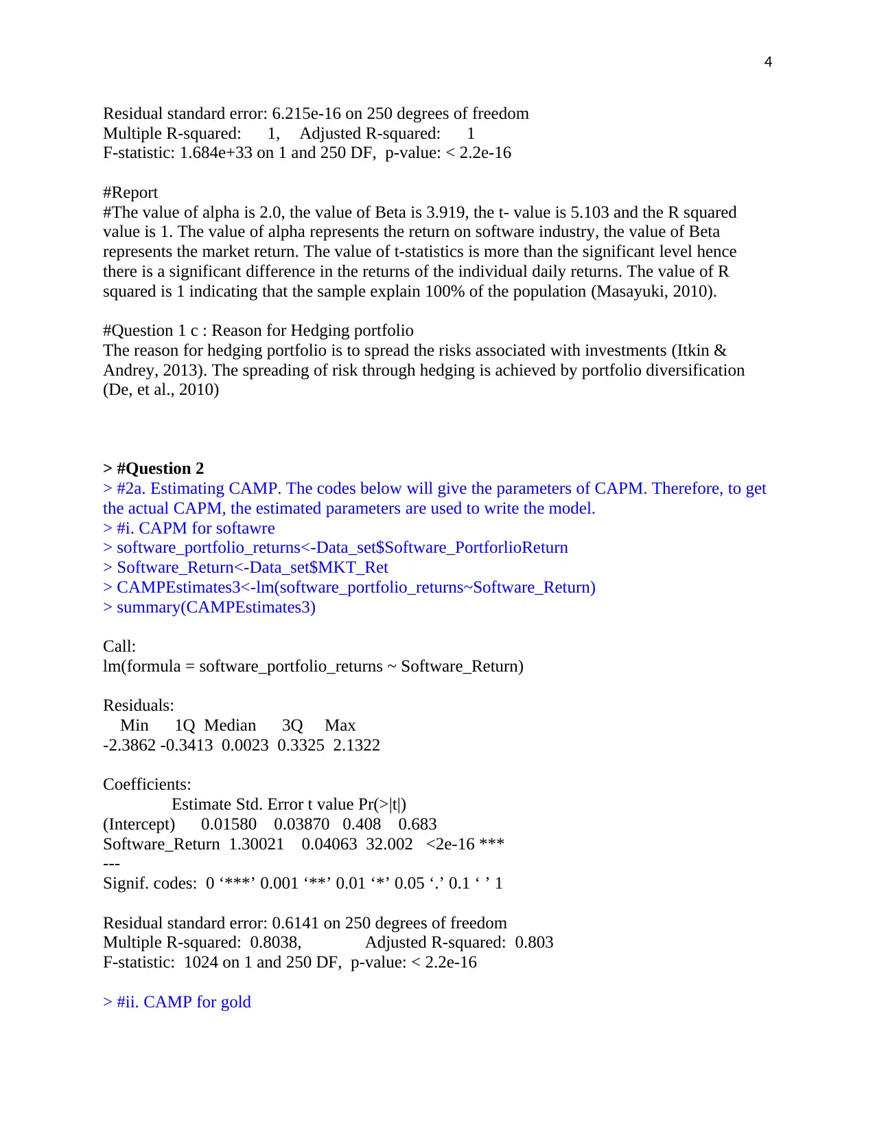
#Report
#The value of alpha is 2.0, the value of Beta is 3.919, the t- value is 5.103 and the R squared
value is 1. The value of alpha represents the return on software industry, the value of Beta
represents the market return. The value of t-statistics is more than the significant level hence
there is a significant difference in the returns of the individual daily returns. The value of R
squared is 1 indicating that the sample explain 100% of the population (Masayuki, 2010).
#Question 1 c : Reason for Hedging portfolio
The reason for hedging portfolio is to spread the risks associated with investments (Itkin &
Andrey, 2013). The spreading of risk through hedging is achieved by portfolio diversification
(De, et al., 2010)
> #Question 2
> #2a. Estimating CAMP. The codes below will give the parameters of CAPM. Therefore, to get
the actual CAPM, the estimated parameters are used to write the model.
> #i. CAPM for softawre
> software_portfolio_returns<-Data_set$Software_PortforlioReturn
> Software_Return<-Data_set$MKT_Ret
> CAMPEstimates3<-lm(software_portfolio_returns~Software_Return)
> summary(CAMPEstimates3)
Call:
lm(formula = software_portfolio_returns ~ Software_Return)
Residuals:
Min 1Q Median 3Q Max
-2.3862 -0.3413 0.0023 0.3325 2.1322
Coefficients:
Estimate Std. Error t value Pr(>|t|)
(Intercept) 0.01580 0.03870 0.408 0.683
Software_Return 1.30021 0.04063 32.002 <2e-16 ***
---
Signif. codes: 0 ‘***’ 0.001 ‘**’ 0.01 ‘*’ 0.05 ‘.’ 0.1 ‘ ’ 1
Residual standard error: 0.6141 on 250 degrees of freedom
Multiple R-squared: 0.8038, Adjusted R-squared: 0.803
F-statistic: 1024 on 1 and 250 DF, p-value: < 2.2e-16
> #ii. CAMP for gold
Residual standard error: 6.215e-16 on 250 degrees of freedom
Multiple R-squared: 1, Adjusted R-squared: 1
F-statistic: 1.684e+33 on 1 and 250 DF, p-value: < 2.2e-16
#Report
#The value of alpha is 2.0, the value of Beta is 3.919, the t- value is 5.103 and the R squared
value is 1. The value of alpha represents the return on software industry, the value of Beta
represents the market return. The value of t-statistics is more than the significant level hence
there is a significant difference in the returns of the individual daily returns. The value of R
squared is 1 indicating that the sample explain 100% of the population (Masayuki, 2010).
#Question 1 c : Reason for Hedging portfolio
The reason for hedging portfolio is to spread the risks associated with investments (Itkin &
Andrey, 2013). The spreading of risk through hedging is achieved by portfolio diversification
(De, et al., 2010)
> #Question 2
> #2a. Estimating CAMP. The codes below will give the parameters of CAPM. Therefore, to get
the actual CAPM, the estimated parameters are used to write the model.
> #i. CAPM for softawre
> software_portfolio_returns<-Data_set$Software_PortforlioReturn
> Software_Return<-Data_set$MKT_Ret
> CAMPEstimates3<-lm(software_portfolio_returns~Software_Return)
> summary(CAMPEstimates3)
Call:
lm(formula = software_portfolio_returns ~ Software_Return)
Residuals:
Min 1Q Median 3Q Max
-2.3862 -0.3413 0.0023 0.3325 2.1322
Coefficients:
Estimate Std. Error t value Pr(>|t|)
(Intercept) 0.01580 0.03870 0.408 0.683
Software_Return 1.30021 0.04063 32.002 <2e-16 ***
---
Signif. codes: 0 ‘***’ 0.001 ‘**’ 0.01 ‘*’ 0.05 ‘.’ 0.1 ‘ ’ 1
Residual standard error: 0.6141 on 250 degrees of freedom
Multiple R-squared: 0.8038, Adjusted R-squared: 0.803
F-statistic: 1024 on 1 and 250 DF, p-value: < 2.2e-16
> #ii. CAMP for gold
Paraphrase This Document
Need a fresh take? Get an instant paraphrase of this document with our AI Paraphraser
5
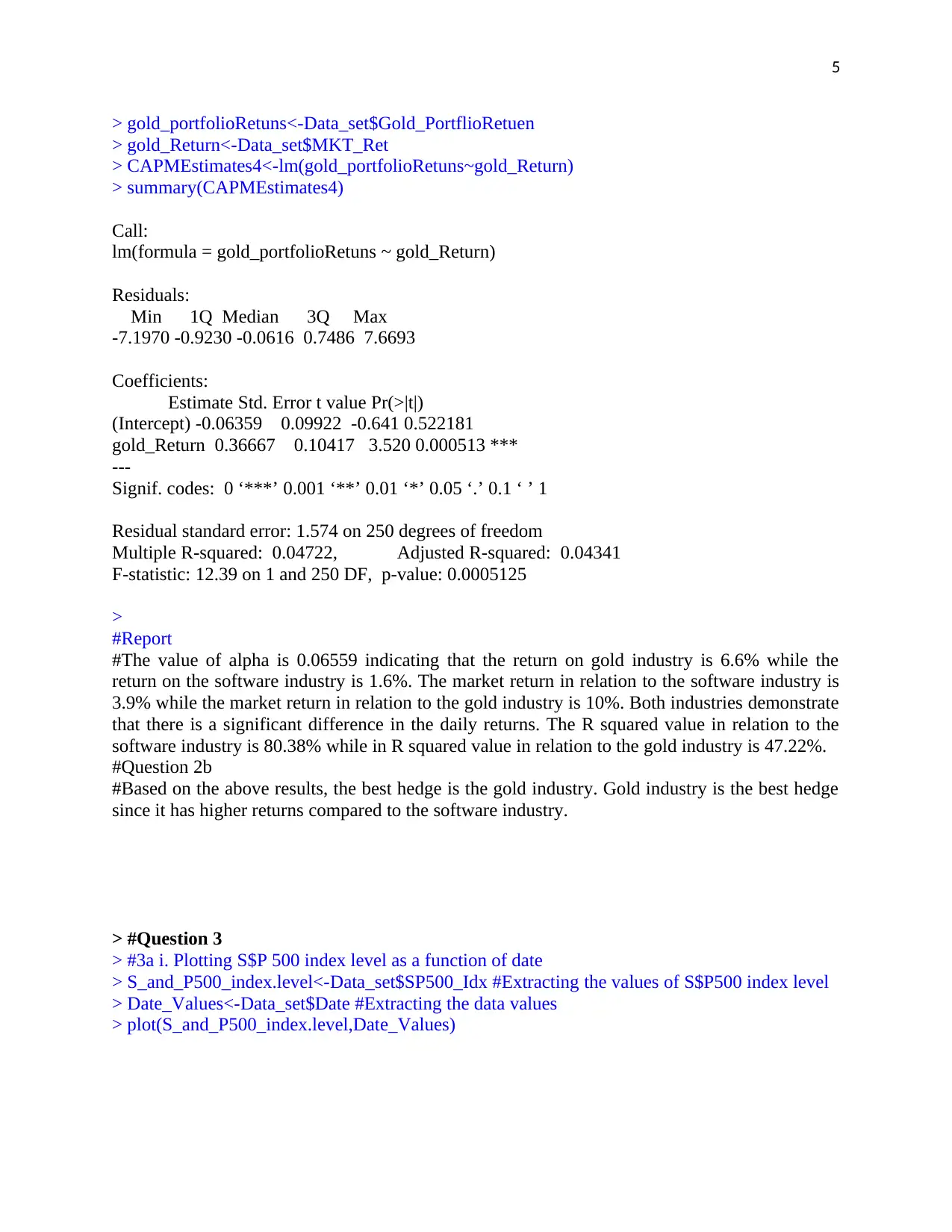
> gold_portfolioRetuns<-Data_set$Gold_PortflioRetuen
> gold_Return<-Data_set$MKT_Ret
> CAPMEstimates4<-lm(gold_portfolioRetuns~gold_Return)
> summary(CAPMEstimates4)
Call:
lm(formula = gold_portfolioRetuns ~ gold_Return)
Residuals:
Min 1Q Median 3Q Max
-7.1970 -0.9230 -0.0616 0.7486 7.6693
Coefficients:
Estimate Std. Error t value Pr(>|t|)
(Intercept) -0.06359 0.09922 -0.641 0.522181
gold_Return 0.36667 0.10417 3.520 0.000513 ***
---
Signif. codes: 0 ‘***’ 0.001 ‘**’ 0.01 ‘*’ 0.05 ‘.’ 0.1 ‘ ’ 1
Residual standard error: 1.574 on 250 degrees of freedom
Multiple R-squared: 0.04722, Adjusted R-squared: 0.04341
F-statistic: 12.39 on 1 and 250 DF, p-value: 0.0005125
>
#Report
#The value of alpha is 0.06559 indicating that the return on gold industry is 6.6% while the
return on the software industry is 1.6%. The market return in relation to the software industry is
3.9% while the market return in relation to the gold industry is 10%. Both industries demonstrate
that there is a significant difference in the daily returns. The R squared value in relation to the
software industry is 80.38% while in R squared value in relation to the gold industry is 47.22%.
#Question 2b
#Based on the above results, the best hedge is the gold industry. Gold industry is the best hedge
since it has higher returns compared to the software industry.
> #Question 3
> #3a i. Plotting S$P 500 index level as a function of date
> S_and_P500_index.level<-Data_set$SP500_Idx #Extracting the values of S$P500 index level
> Date_Values<-Data_set$Date #Extracting the data values
> plot(S_and_P500_index.level,Date_Values)
6
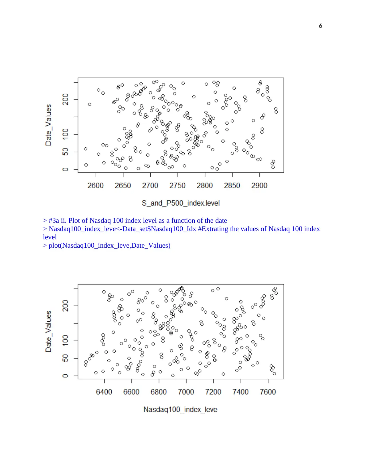
> #3a ii. Plot of Nasdaq 100 index level as a function of the date
> Nasdaq100_index_leve<-Data_set$Nasdaq100_Idx #Extrating the values of Nasdaq 100 index
level
> plot(Nasdaq100_index_leve,Date_Values)
> #3a ii. Plot of Nasdaq 100 index level as a function of the date
> Nasdaq100_index_leve<-Data_set$Nasdaq100_Idx #Extrating the values of Nasdaq 100 index
level
> plot(Nasdaq100_index_leve,Date_Values)
⊘ This is a preview!⊘
Do you want full access?
Subscribe today to unlock all pages.
Trusted by 1+ million students worldwide
7
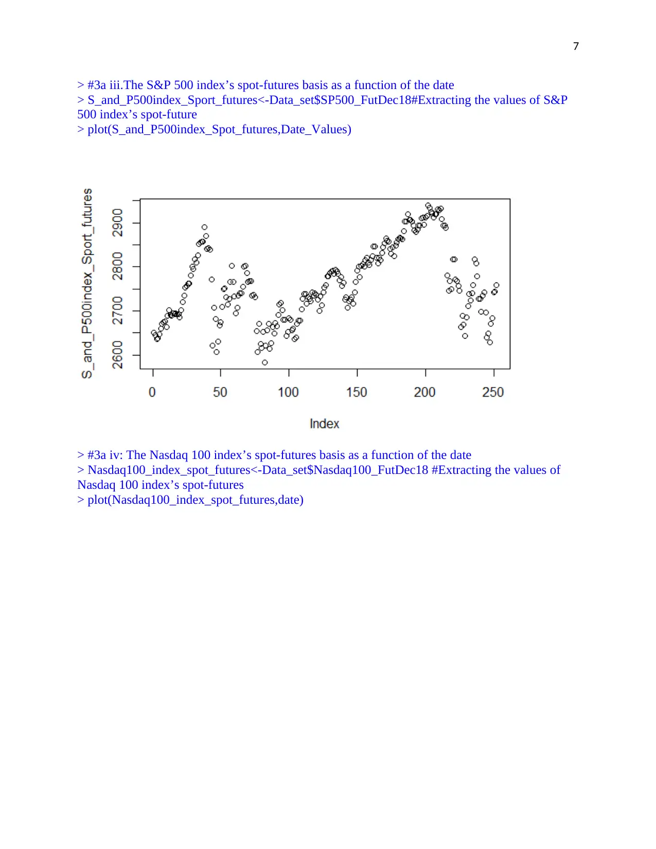
> #3a iii.The S&P 500 index’s spot-futures basis as a function of the date
> S_and_P500index_Sport_futures<-Data_set$SP500_FutDec18#Extracting the values of S&P
500 index’s spot-future
> plot(S_and_P500index_Spot_futures,Date_Values)
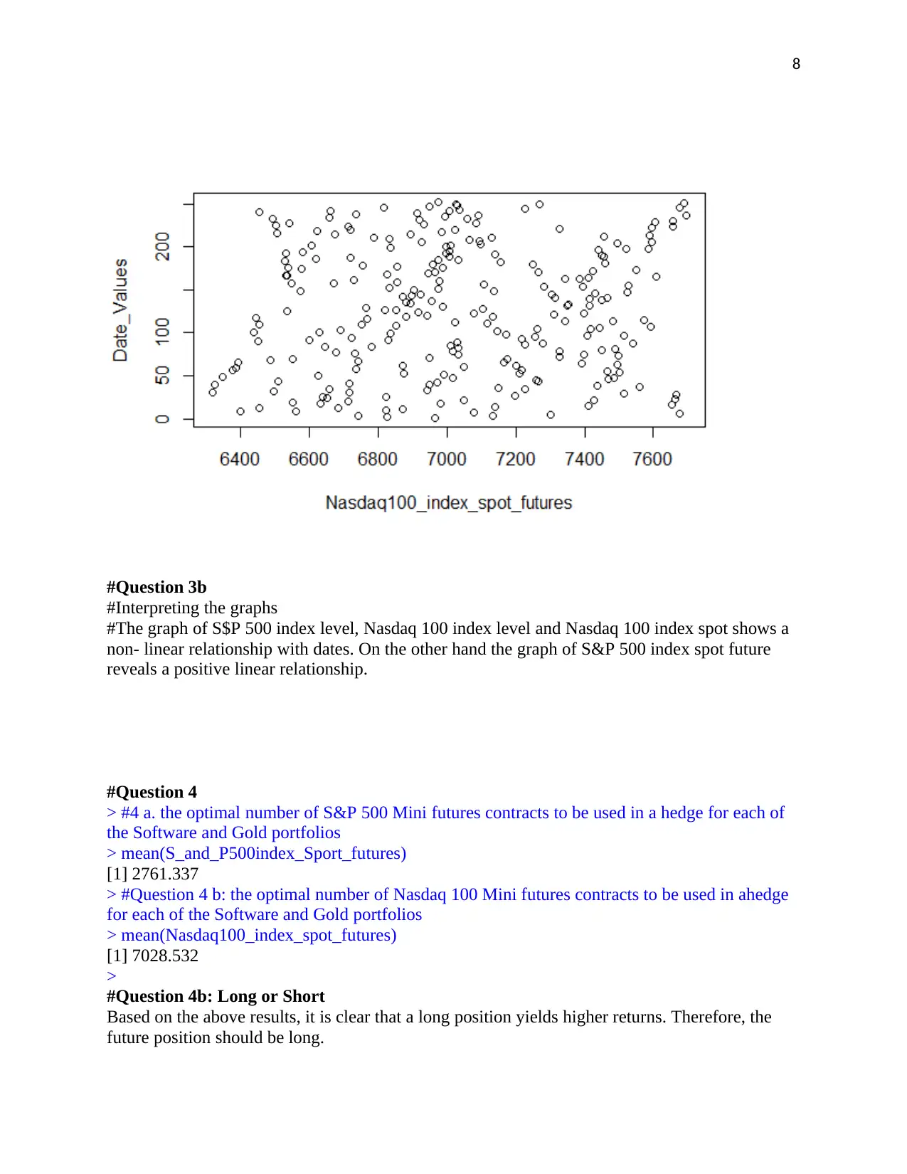
> #3a iv: The Nasdaq 100 index’s spot-futures basis as a function of the date
> Nasdaq100_index_spot_futures<-Data_set$Nasdaq100_FutDec18 #Extracting the values of
Nasdaq 100 index’s spot-futures
> plot(Nasdaq100_index_spot_futures,date)
> #3a iii.The S&P 500 index’s spot-futures basis as a function of the date
> S_and_P500index_Sport_futures<-Data_set$SP500_FutDec18#Extracting the values of S&P
500 index’s spot-future
> plot(S_and_P500index_Spot_futures,Date_Values)
> #3a iv: The Nasdaq 100 index’s spot-futures basis as a function of the date
> Nasdaq100_index_spot_futures<-Data_set$Nasdaq100_FutDec18 #Extracting the values of
Nasdaq 100 index’s spot-futures
> plot(Nasdaq100_index_spot_futures,date)
Paraphrase This Document
Need a fresh take? Get an instant paraphrase of this document with our AI Paraphraser
8
#Question 3b
#Interpreting the graphs
#The graph of S$P 500 index level, Nasdaq 100 index level and Nasdaq 100 index spot shows a
non- linear relationship with dates. On the other hand the graph of S&P 500 index spot future
reveals a positive linear relationship.
#Question 4
> #4 a. the optimal number of S&P 500 Mini futures contracts to be used in a hedge for each of
the Software and Gold portfolios
> mean(S_and_P500index_Sport_futures)
[1] 2761.337
> #Question 4 b: the optimal number of Nasdaq 100 Mini futures contracts to be used in ahedge
for each of the Software and Gold portfolios
> mean(Nasdaq100_index_spot_futures)
[1] 7028.532
>
#Question 4b: Long or Short
Based on the above results, it is clear that a long position yields higher returns. Therefore, the
future position should be long.
9
> #Question 5
> #5 a:Cumulative gain on the Software portfolio is hedged using the S&P 500 Mini
> Day_gain<-1
> Software_size<-Data_set$Softw_Ret
> N<-Software_size[20]
> future_return<-Data_set$RF
> F0<-future_return[19]
> F1<-future_return[152]
> S_and_P500Mini<-Data_set$SP500_Ret
> S<-S_and_P500Mini[152]
> Cumulative_gain1<-Day_gain*N*S*(F1-F0)
> Cumulative_gain1
[1] 0.001220199
>
> #5b the Software portfolio is hedged using the Nasdaq 100 Mini,
> Software_size<-Data_set$Softw_Ret
> N<-Software_size[20]
> future_return<-Data_set$RF
> F00<-future_return[19]
> F11<-future_return[152]
> Nasda100_mini<-Data_set$Nasdaq100_Ret
> S1<-Nasda100_mini[152]
> Cumulative_gain2<-Day_gain*N1*S1*(F1-F0)
> mean(Cumulative_gain2)
[1] -0.0303062
>
> #5c the Gold portfolio is hedged using the S&P 500 Mini
>
> Day_gain<-1
> gold_size<-Data_set$Gold_Ret
> N<-gold_size[20]
> future_return<-Data_set$RF
> F0<-future_return[19]
> F1<-future_return[152]
> S_and_P500Mini<-Data_set$SP500_Ret
> S<-S_and_P500Mini[152]
> Cumulative_gain3<-Day_gain*N*S*(F1-F0)
> Cumulative_gain3
[1] 0.0001135069
>
> # 5D: the Gold portfolio is hedged using the Nasdaq 100 Mini.
> N<-gold_size[20]
> future_return<-Data_set$RF
> F00<-future_return[19]
⊘ This is a preview!⊘
Do you want full access?
Subscribe today to unlock all pages.
Trusted by 1+ million students worldwide
10
> F11<-future_return[152]
> Nasda100_mini<-Data_set$Nasdaq100_Ret
> S1<-Nasda100_mini[152]
> Cumulative_gain4<-Day_gain*N1*S1*(F1-F0)
> mean(Cumulative_gain4)
[1] -0.0303062
>
#Report
Therefore the cumulative gains are:
For 29 Dec 2017 the cumulative gain is 0.001221, for 29 June 2018 the cumulative gain is -
0.030306 and for 30 November 2018, the cumulative gain is 0.001138069.
> #Question 6
> #A. Hedged portfolio
> hedged_portfolio1<-Software_size[20]+Cumulative_gain
> hedged_portfolio1
[1] -0.428217
> #b
> hedged_portfolio2<-Software_size[20]+Cumulative_gain1
> hedged_portfolio2
[1] -0.4287798
> #c
> hedged_portfolio3<-gold_size[20]+Cumulative_gain3
> hedged_portfolio3
[1] -0.03988649
> #d
> hedged_portfolio4<-gold_size[20]+Cumulative_gain4
>
> #6B
> #the value of the hedged portfolio position on the following three dates: i) 29 December 2017,
ii) 29 June 2018, and iii) 30 November 2018.
> #a
> hedged_position_dec2017<-Software_size[20]+Cumulative_gain
> hedged_position_dec2017
[1] -0.428217
> hedged_position_june2018<-Software_size[145]+Cumulative_gain
> hedged_position_june2018
[1] 0.05178301
Paraphrase This Document
Need a fresh take? Get an instant paraphrase of this document with our AI Paraphraser
11
> hedged_position_nov2018<-Software_size[252]+Cumulative_gain
> hedged_position_nov2018
[1] 1.011783
> #b
> hedged_position_dec2017_1<-Software_size[20]+Cumulative_gain1
> hedged_position_dec2017_1
[1] -0.4287798
> hedged_position_june2018_1<-Software_size[145]+Cumulative_gain1
> hedged_position_june2018_1
[1] 0.0512202
> hedged_position_nov2018_1<-Software_size[252]+Cumulative_gain1
> hedged_position_nov2018_1
[1] 1.01122
> #c
> hedged_position_dec2017_2<-Software_size[20]+Cumulative_gain3
> hedged_position_dec2017_2
[1] -0.4298865
> hedged_position_june2018_2<-Software_size[145]+Cumulative_gain3
> hedged_position_june2018_2
[1] 0.05011351
> hedged_position_nov2018_2<-Software_size[252]+Cumulative_gain3
> mean(hedged_position_nov2018_2)
[1] 1.010114
> #d
> hedged_position_dec2017_3<-Software_size[20]+Cumulative_gain4
> mean(hedged_position_dec2017_3)
[1] -0.4603062
> hedged_position_june2018_3<-Software_size[145]+Cumulative_gain4
> hedged_position_june2018
[1] 0.05178301
> hedged_position_nov2018_3<-Software_size[252]+Cumulative_gain4
> mean(hedged_position_nov2018_3)
[1] 0.9796938
>
12
#Report
#Report
⊘ This is a preview!⊘
Do you want full access?
Subscribe today to unlock all pages.
Trusted by 1+ million students worldwide
1 out of 26
Related Documents


Your All-in-One AI-Powered Toolkit for Academic Success.
+13062052269
info@desklib.com
Available 24*7 on WhatsApp / Email
![[object Object]](/_next/static/media/star-bottom.7253800d.svg)
Unlock your academic potential
Copyright © 2020–2026 A2Z Services. All Rights Reserved. Developed and managed by ZUCOL.