University Finance Assignment: Eviews Analysis of Time Series Data
VerifiedAdded on 2020/05/28
|31
|5859
|216
Homework Assignment
AI Summary
This finance assignment focuses on time series analysis using Eviews software. The analysis begins with an examination of the G10 series, including its trends and fluctuations. The assignment then delves into testing whether the G10 variable follows a martingale process, employing both Chow-Denning and Wild Bootstrap tests. The order of integration is determined using correlograms and Augmented Dickey-Fuller (ADF) tests. The ADF test is performed with different specifications to confirm the order of integration. Further analysis includes the examination of cointegration and the development of an error correction model. The solution provides detailed regression outputs, test statistics, and interpretations to support the conclusions drawn about the time series properties of the data.
Running Head: FINANCE WITH EVIEWS
Finance with Eviews
Name of the Student
Name of the University
Author note
Finance with Eviews
Name of the Student
Name of the University
Author note
Paraphrase This Document
Need a fresh take? Get an instant paraphrase of this document with our AI Paraphraser
1
FINANCE WITH EVIEWS
Table of Contents
Answer 1..........................................................................................................................................2
Answer 2..........................................................................................................................................3
Martingale test.............................................................................................................................4
Answer 3..........................................................................................................................................6
Answer 4........................................................................................................................................16
Order of integration for SPREAD.............................................................................................16
Co-integration test.....................................................................................................................22
Answer 5........................................................................................................................................27
Error Correction Model.............................................................................................................27
2
FINANCE WITH EVIEWS
Answer 1
0
2
4
6
8
10
12
14
16
60 65 70 75 80 85 90 95 00 05 10
G10
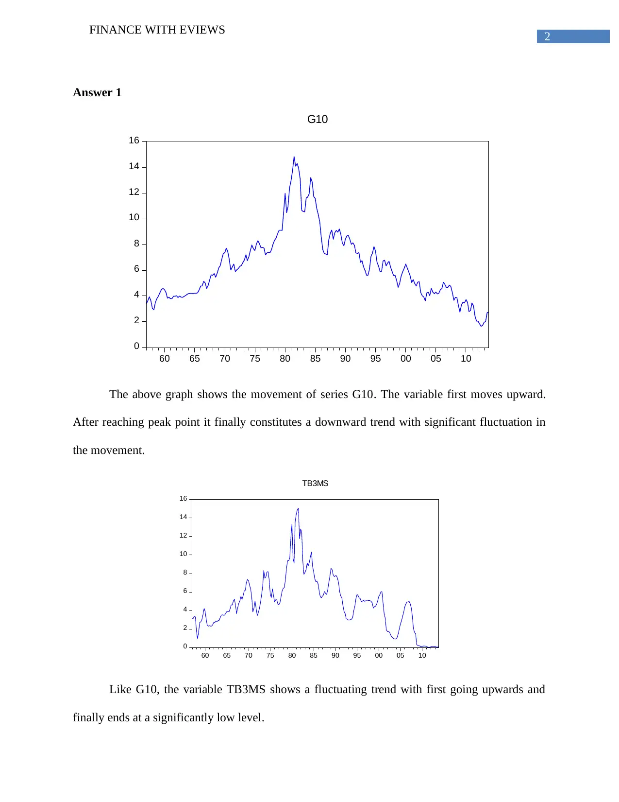
The above graph shows the movement of series G10. The variable first moves upward.
After reaching peak point it finally constitutes a downward trend with significant fluctuation in
the movement.
0
2
4
6
8
10
12
14
16
60 65 70 75 80 85 90 95 00 05 10
TB3MS
Like G10, the variable TB3MS shows a fluctuating trend with first going upwards and
finally ends at a significantly low level.
FINANCE WITH EVIEWS
Answer 1
0
2
4
6
8
10
12
14
16
60 65 70 75 80 85 90 95 00 05 10
G10
The above graph shows the movement of series G10. The variable first moves upward.
After reaching peak point it finally constitutes a downward trend with significant fluctuation in
the movement.
0
2
4
6
8
10
12
14
16
60 65 70 75 80 85 90 95 00 05 10
TB3MS
Like G10, the variable TB3MS shows a fluctuating trend with first going upwards and
finally ends at a significantly low level.
⊘ This is a preview!⊘
Do you want full access?
Subscribe today to unlock all pages.
Trusted by 1+ million students worldwide
3
FINANCE WITH EVIEWS
Answer 2
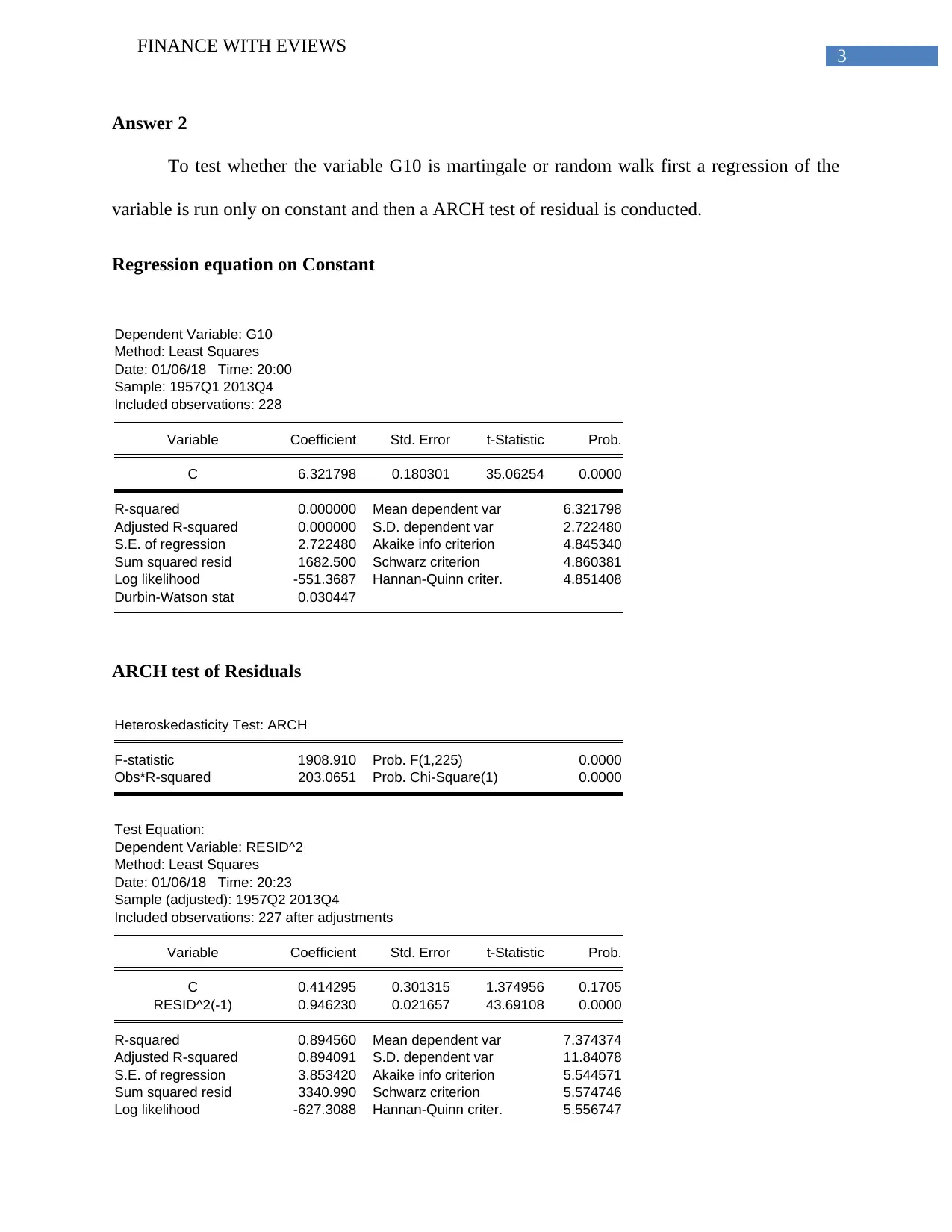
To test whether the variable G10 is martingale or random walk first a regression of the
variable is run only on constant and then a ARCH test of residual is conducted.
Regression equation on Constant
Dependent Variable: G10
Method: Least Squares
Date: 01/06/18 Time: 20:00
Sample: 1957Q1 2013Q4
Included observations: 228
Variable Coefficient Std. Error t-Statistic Prob.
C 6.321798 0.180301 35.06254 0.0000
R-squared 0.000000 Mean dependent var 6.321798
Adjusted R-squared 0.000000 S.D. dependent var 2.722480
S.E. of regression 2.722480 Akaike info criterion 4.845340
Sum squared resid 1682.500 Schwarz criterion 4.860381
Log likelihood -551.3687 Hannan-Quinn criter. 4.851408
Durbin-Watson stat 0.030447
ARCH test of Residuals
Heteroskedasticity Test: ARCH
F-statistic 1908.910 Prob. F(1,225) 0.0000
Obs*R-squared 203.0651 Prob. Chi-Square(1) 0.0000
Test Equation:
Dependent Variable: RESID^2
Method: Least Squares
Date: 01/06/18 Time: 20:23
Sample (adjusted): 1957Q2 2013Q4
Included observations: 227 after adjustments
Variable Coefficient Std. Error t-Statistic Prob.
C 0.414295 0.301315 1.374956 0.1705
RESID^2(-1) 0.946230 0.021657 43.69108 0.0000
R-squared 0.894560 Mean dependent var 7.374374
Adjusted R-squared 0.894091 S.D. dependent var 11.84078
S.E. of regression 3.853420 Akaike info criterion 5.544571
Sum squared resid 3340.990 Schwarz criterion 5.574746
Log likelihood -627.3088 Hannan-Quinn criter. 5.556747
FINANCE WITH EVIEWS
Answer 2
To test whether the variable G10 is martingale or random walk first a regression of the
variable is run only on constant and then a ARCH test of residual is conducted.
Regression equation on Constant
Dependent Variable: G10
Method: Least Squares
Date: 01/06/18 Time: 20:00
Sample: 1957Q1 2013Q4
Included observations: 228
Variable Coefficient Std. Error t-Statistic Prob.
C 6.321798 0.180301 35.06254 0.0000
R-squared 0.000000 Mean dependent var 6.321798
Adjusted R-squared 0.000000 S.D. dependent var 2.722480
S.E. of regression 2.722480 Akaike info criterion 4.845340
Sum squared resid 1682.500 Schwarz criterion 4.860381
Log likelihood -551.3687 Hannan-Quinn criter. 4.851408
Durbin-Watson stat 0.030447
ARCH test of Residuals
Heteroskedasticity Test: ARCH
F-statistic 1908.910 Prob. F(1,225) 0.0000
Obs*R-squared 203.0651 Prob. Chi-Square(1) 0.0000
Test Equation:
Dependent Variable: RESID^2
Method: Least Squares
Date: 01/06/18 Time: 20:23
Sample (adjusted): 1957Q2 2013Q4
Included observations: 227 after adjustments
Variable Coefficient Std. Error t-Statistic Prob.
C 0.414295 0.301315 1.374956 0.1705
RESID^2(-1) 0.946230 0.021657 43.69108 0.0000
R-squared 0.894560 Mean dependent var 7.374374
Adjusted R-squared 0.894091 S.D. dependent var 11.84078
S.E. of regression 3.853420 Akaike info criterion 5.544571
Sum squared resid 3340.990 Schwarz criterion 5.574746
Log likelihood -627.3088 Hannan-Quinn criter. 5.556747
Paraphrase This Document
Need a fresh take? Get an instant paraphrase of this document with our AI Paraphraser
4
FINANCE WITH EVIEWS
F-statistic 1908.910 Durbin-Watson stat 1.563370
Prob(F-statistic) 0.000000
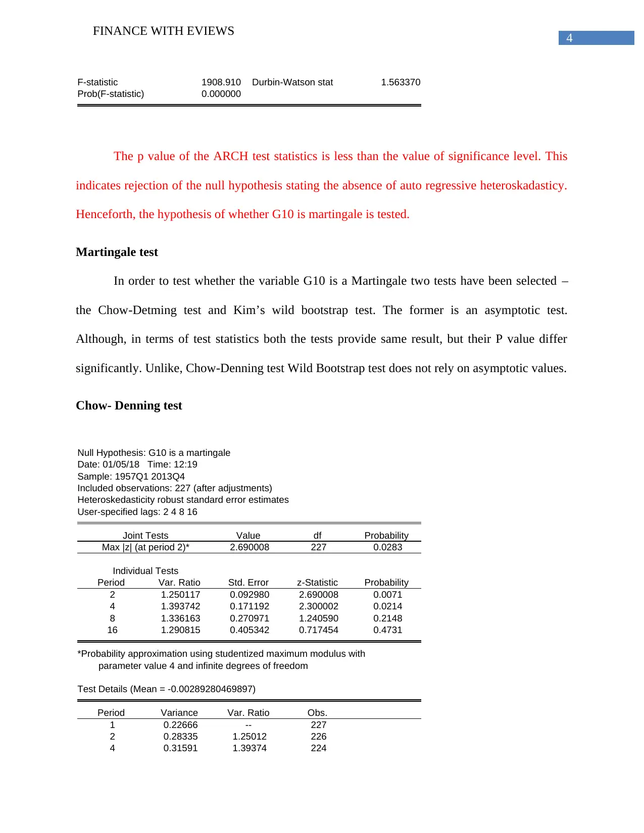
The p value of the ARCH test statistics is less than the value of significance level. This
indicates rejection of the null hypothesis stating the absence of auto regressive heteroskadasticy.
Henceforth, the hypothesis of whether G10 is martingale is tested.
Martingale test
In order to test whether the variable G10 is a Martingale two tests have been selected –
the Chow-Detming test and Kim’s wild bootstrap test. The former is an asymptotic test.
Although, in terms of test statistics both the tests provide same result, but their P value differ
significantly. Unlike, Chow-Denning test Wild Bootstrap test does not rely on asymptotic values.
Chow- Denning test
Null Hypothesis: G10 is a martingale
Date: 01/05/18 Time: 12:19
Sample: 1957Q1 2013Q4
Included observations: 227 (after adjustments)
Heteroskedasticity robust standard error estimates
User-specified lags: 2 4 8 16
Joint Tests Value df Probability
Max |z| (at period 2)* 2.690008 227 0.0283
Individual Tests
Period Var. Ratio Std. Error z-Statistic Probability
2 1.250117 0.092980 2.690008 0.0071
4 1.393742 0.171192 2.300002 0.0214
8 1.336163 0.270971 1.240590 0.2148
16 1.290815 0.405342 0.717454 0.4731
*Probability approximation using studentized maximum modulus with
parameter value 4 and infinite degrees of freedom
Test Details (Mean = -0.00289280469897)
Period Variance Var. Ratio Obs.
1 0.22666 -- 227
2 0.28335 1.25012 226
4 0.31591 1.39374 224
FINANCE WITH EVIEWS
F-statistic 1908.910 Durbin-Watson stat 1.563370
Prob(F-statistic) 0.000000
The p value of the ARCH test statistics is less than the value of significance level. This
indicates rejection of the null hypothesis stating the absence of auto regressive heteroskadasticy.
Henceforth, the hypothesis of whether G10 is martingale is tested.
Martingale test
In order to test whether the variable G10 is a Martingale two tests have been selected –
the Chow-Detming test and Kim’s wild bootstrap test. The former is an asymptotic test.
Although, in terms of test statistics both the tests provide same result, but their P value differ
significantly. Unlike, Chow-Denning test Wild Bootstrap test does not rely on asymptotic values.
Chow- Denning test
Null Hypothesis: G10 is a martingale
Date: 01/05/18 Time: 12:19
Sample: 1957Q1 2013Q4
Included observations: 227 (after adjustments)
Heteroskedasticity robust standard error estimates
User-specified lags: 2 4 8 16
Joint Tests Value df Probability
Max |z| (at period 2)* 2.690008 227 0.0283
Individual Tests
Period Var. Ratio Std. Error z-Statistic Probability
2 1.250117 0.092980 2.690008 0.0071
4 1.393742 0.171192 2.300002 0.0214
8 1.336163 0.270971 1.240590 0.2148
16 1.290815 0.405342 0.717454 0.4731
*Probability approximation using studentized maximum modulus with
parameter value 4 and infinite degrees of freedom
Test Details (Mean = -0.00289280469897)
Period Variance Var. Ratio Obs.
1 0.22666 -- 227
2 0.28335 1.25012 226
4 0.31591 1.39374 224
5
FINANCE WITH EVIEWS
8 0.30286 1.33616 220
16 0.29258 1.29081 212
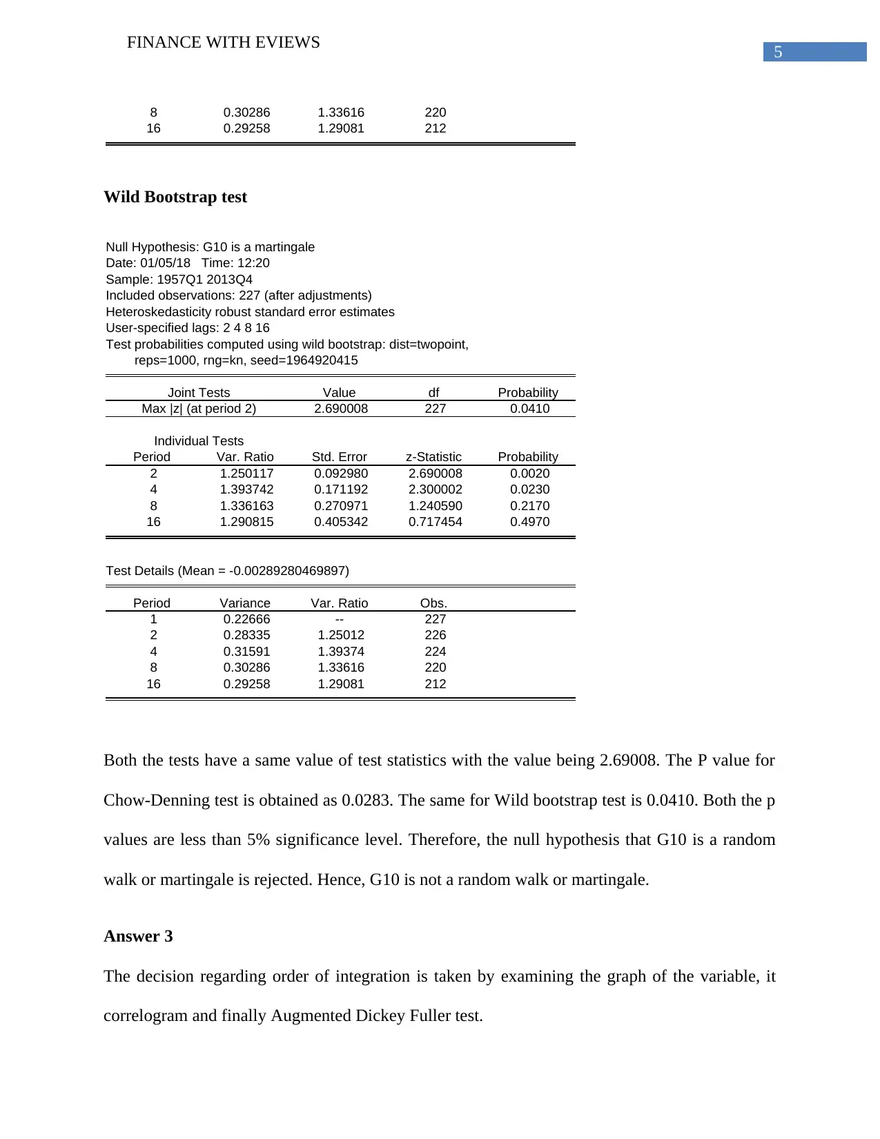
Wild Bootstrap test
Null Hypothesis: G10 is a martingale
Date: 01/05/18 Time: 12:20
Sample: 1957Q1 2013Q4
Included observations: 227 (after adjustments)
Heteroskedasticity robust standard error estimates
User-specified lags: 2 4 8 16
Test probabilities computed using wild bootstrap: dist=twopoint,
reps=1000, rng=kn, seed=1964920415
Joint Tests Value df Probability
Max |z| (at period 2) 2.690008 227 0.0410
Individual Tests
Period Var. Ratio Std. Error z-Statistic Probability
2 1.250117 0.092980 2.690008 0.0020
4 1.393742 0.171192 2.300002 0.0230
8 1.336163 0.270971 1.240590 0.2170
16 1.290815 0.405342 0.717454 0.4970
Test Details (Mean = -0.00289280469897)
Period Variance Var. Ratio Obs.
1 0.22666 -- 227
2 0.28335 1.25012 226
4 0.31591 1.39374 224
8 0.30286 1.33616 220
16 0.29258 1.29081 212
Both the tests have a same value of test statistics with the value being 2.69008. The P value for
Chow-Denning test is obtained as 0.0283. The same for Wild bootstrap test is 0.0410. Both the p
values are less than 5% significance level. Therefore, the null hypothesis that G10 is a random
walk or martingale is rejected. Hence, G10 is not a random walk or martingale.
Answer 3
The decision regarding order of integration is taken by examining the graph of the variable, it
correlogram and finally Augmented Dickey Fuller test.
FINANCE WITH EVIEWS
8 0.30286 1.33616 220
16 0.29258 1.29081 212
Wild Bootstrap test
Null Hypothesis: G10 is a martingale
Date: 01/05/18 Time: 12:20
Sample: 1957Q1 2013Q4
Included observations: 227 (after adjustments)
Heteroskedasticity robust standard error estimates
User-specified lags: 2 4 8 16
Test probabilities computed using wild bootstrap: dist=twopoint,
reps=1000, rng=kn, seed=1964920415
Joint Tests Value df Probability
Max |z| (at period 2) 2.690008 227 0.0410
Individual Tests
Period Var. Ratio Std. Error z-Statistic Probability
2 1.250117 0.092980 2.690008 0.0020
4 1.393742 0.171192 2.300002 0.0230
8 1.336163 0.270971 1.240590 0.2170
16 1.290815 0.405342 0.717454 0.4970
Test Details (Mean = -0.00289280469897)
Period Variance Var. Ratio Obs.
1 0.22666 -- 227
2 0.28335 1.25012 226
4 0.31591 1.39374 224
8 0.30286 1.33616 220
16 0.29258 1.29081 212
Both the tests have a same value of test statistics with the value being 2.69008. The P value for
Chow-Denning test is obtained as 0.0283. The same for Wild bootstrap test is 0.0410. Both the p
values are less than 5% significance level. Therefore, the null hypothesis that G10 is a random
walk or martingale is rejected. Hence, G10 is not a random walk or martingale.
Answer 3
The decision regarding order of integration is taken by examining the graph of the variable, it
correlogram and finally Augmented Dickey Fuller test.
⊘ This is a preview!⊘
Do you want full access?
Subscribe today to unlock all pages.
Trusted by 1+ million students worldwide
6
FINANCE WITH EVIEWS
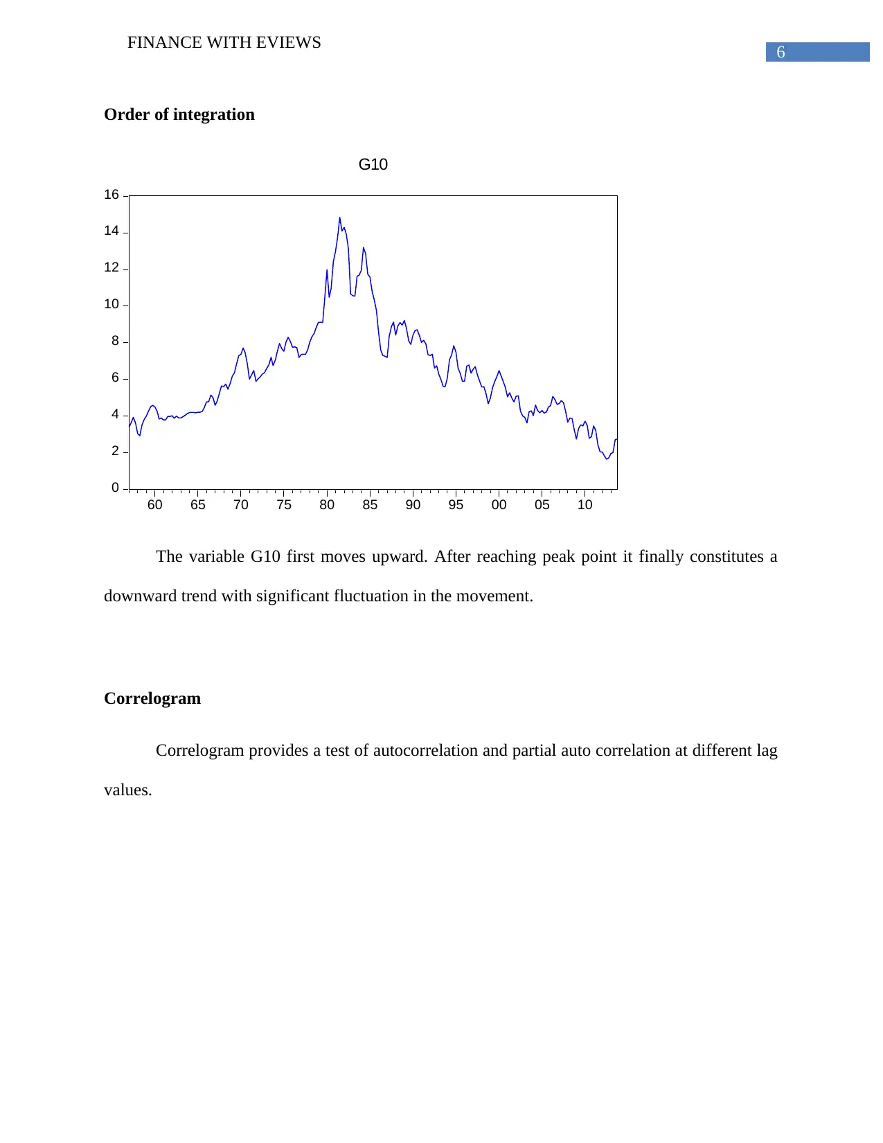
Order of integration
0
2
4
6
8
10
12
14
16
60 65 70 75 80 85 90 95 00 05 10
G10
The variable G10 first moves upward. After reaching peak point it finally constitutes a
downward trend with significant fluctuation in the movement.
Correlogram
Correlogram provides a test of autocorrelation and partial auto correlation at different lag
values.
FINANCE WITH EVIEWS
Order of integration
0
2
4
6
8
10
12
14
16
60 65 70 75 80 85 90 95 00 05 10
G10
The variable G10 first moves upward. After reaching peak point it finally constitutes a
downward trend with significant fluctuation in the movement.
Correlogram
Correlogram provides a test of autocorrelation and partial auto correlation at different lag
values.
Paraphrase This Document
Need a fresh take? Get an instant paraphrase of this document with our AI Paraphraser
7
FINANCE WITH EVIEWS
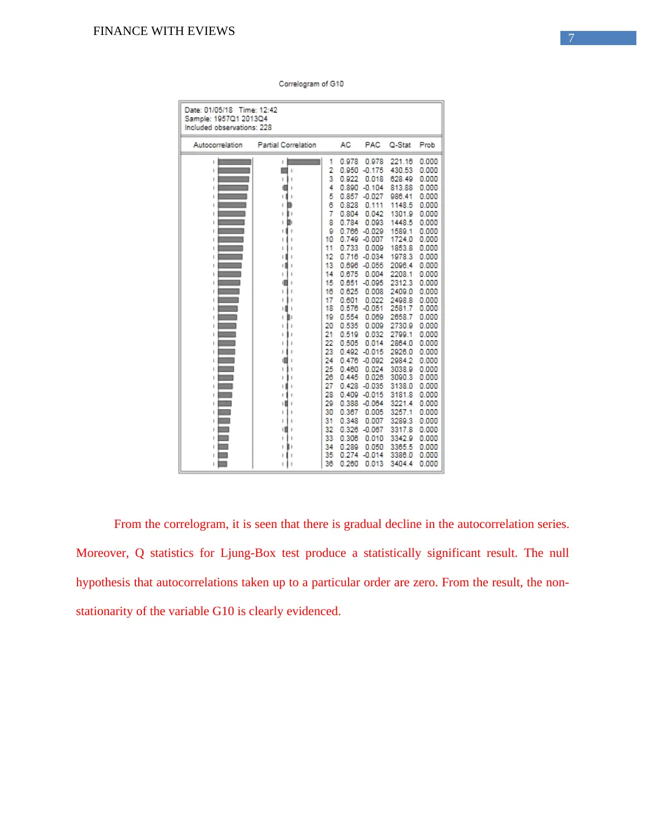
From the correlogram, it is seen that there is gradual decline in the autocorrelation series.
Moreover, Q statistics for Ljung-Box test produce a statistically significant result. The null
hypothesis that autocorrelations taken up to a particular order are zero. From the result, the non-
stationarity of the variable G10 is clearly evidenced.
FINANCE WITH EVIEWS
From the correlogram, it is seen that there is gradual decline in the autocorrelation series.
Moreover, Q statistics for Ljung-Box test produce a statistically significant result. The null
hypothesis that autocorrelations taken up to a particular order are zero. From the result, the non-
stationarity of the variable G10 is clearly evidenced.
8
FINANCE WITH EVIEWS
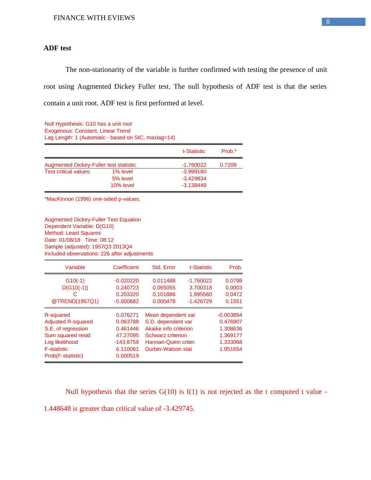
ADF test
The non-stationarity of the variable is further confirmed with testing the presence of unit
root using Augmented Dickey Fuller test. The null hypothesis of ADF test is that the series
contain a unit root. ADF test is first performed at level.
Null Hypothesis: G10 has a unit root
Exogenous: Constant, Linear Trend
Lag Length: 1 (Automatic - based on SIC, maxlag=14)
t-Statistic Prob.*
Augmented Dickey-Fuller test statistic -1.760022 0.7209
Test critical values: 1% level -3.999180
5% level -3.429834
10% level -3.138449
*MacKinnon (1996) one-sided p-values.
Augmented Dickey-Fuller Test Equation
Dependent Variable: D(G10)
Method: Least Squares
Date: 01/08/18 Time: 08:12
Sample (adjusted): 1957Q3 2013Q4
Included observations: 226 after adjustments
Variable Coefficient Std. Error t-Statistic Prob.
G10(-1) -0.020220 0.011488 -1.760022 0.0798
D(G10(-1)) 0.240723 0.065055 3.700318 0.0003
C 0.203320 0.101886 1.995560 0.0472
@TREND(1957Q1) -0.000682 0.000478 -1.426729 0.1551
R-squared 0.076271 Mean dependent var -0.003894
Adjusted R-squared 0.063788 S.D. dependent var 0.476907
S.E. of regression 0.461446 Akaike info criterion 1.308636
Sum squared resid 47.27095 Schwarz criterion 1.369177
Log likelihood -143.8759 Hannan-Quinn criter. 1.333068
F-statistic 6.110061 Durbin-Watson stat 1.951654
Prob(F-statistic) 0.000519
Null hypothesis that the series G(10) is I(1) is not rejected as the t computed t value -
1.448648 is greater than critical value of -3.429745.
FINANCE WITH EVIEWS
ADF test
The non-stationarity of the variable is further confirmed with testing the presence of unit
root using Augmented Dickey Fuller test. The null hypothesis of ADF test is that the series
contain a unit root. ADF test is first performed at level.
Null Hypothesis: G10 has a unit root
Exogenous: Constant, Linear Trend
Lag Length: 1 (Automatic - based on SIC, maxlag=14)
t-Statistic Prob.*
Augmented Dickey-Fuller test statistic -1.760022 0.7209
Test critical values: 1% level -3.999180
5% level -3.429834
10% level -3.138449
*MacKinnon (1996) one-sided p-values.
Augmented Dickey-Fuller Test Equation
Dependent Variable: D(G10)
Method: Least Squares
Date: 01/08/18 Time: 08:12
Sample (adjusted): 1957Q3 2013Q4
Included observations: 226 after adjustments
Variable Coefficient Std. Error t-Statistic Prob.
G10(-1) -0.020220 0.011488 -1.760022 0.0798
D(G10(-1)) 0.240723 0.065055 3.700318 0.0003
C 0.203320 0.101886 1.995560 0.0472
@TREND(1957Q1) -0.000682 0.000478 -1.426729 0.1551
R-squared 0.076271 Mean dependent var -0.003894
Adjusted R-squared 0.063788 S.D. dependent var 0.476907
S.E. of regression 0.461446 Akaike info criterion 1.308636
Sum squared resid 47.27095 Schwarz criterion 1.369177
Log likelihood -143.8759 Hannan-Quinn criter. 1.333068
F-statistic 6.110061 Durbin-Watson stat 1.951654
Prob(F-statistic) 0.000519
Null hypothesis that the series G(10) is I(1) is not rejected as the t computed t value -
1.448648 is greater than critical value of -3.429745.
⊘ This is a preview!⊘
Do you want full access?
Subscribe today to unlock all pages.
Trusted by 1+ million students worldwide
9
FINANCE WITH EVIEWS
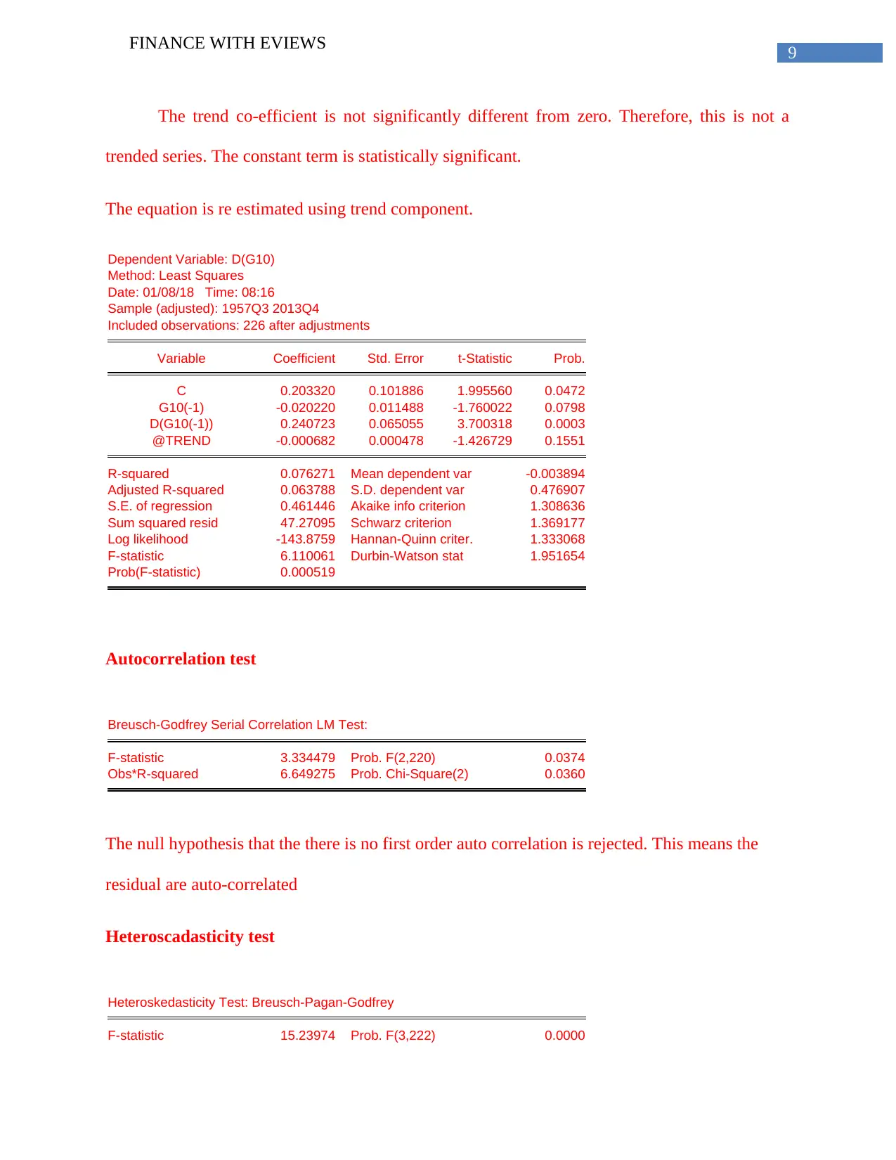
The trend co-efficient is not significantly different from zero. Therefore, this is not a
trended series. The constant term is statistically significant.
The equation is re estimated using trend component.
Dependent Variable: D(G10)
Method: Least Squares
Date: 01/08/18 Time: 08:16
Sample (adjusted): 1957Q3 2013Q4
Included observations: 226 after adjustments
Variable Coefficient Std. Error t-Statistic Prob.
C 0.203320 0.101886 1.995560 0.0472
G10(-1) -0.020220 0.011488 -1.760022 0.0798
D(G10(-1)) 0.240723 0.065055 3.700318 0.0003
@TREND -0.000682 0.000478 -1.426729 0.1551
R-squared 0.076271 Mean dependent var -0.003894
Adjusted R-squared 0.063788 S.D. dependent var 0.476907
S.E. of regression 0.461446 Akaike info criterion 1.308636
Sum squared resid 47.27095 Schwarz criterion 1.369177
Log likelihood -143.8759 Hannan-Quinn criter. 1.333068
F-statistic 6.110061 Durbin-Watson stat 1.951654
Prob(F-statistic) 0.000519
Autocorrelation test
Breusch-Godfrey Serial Correlation LM Test:
F-statistic 3.334479 Prob. F(2,220) 0.0374
Obs*R-squared 6.649275 Prob. Chi-Square(2) 0.0360
The null hypothesis that the there is no first order auto correlation is rejected. This means the
residual are auto-correlated
Heteroscadasticity test
Heteroskedasticity Test: Breusch-Pagan-Godfrey
F-statistic 15.23974 Prob. F(3,222) 0.0000
FINANCE WITH EVIEWS
The trend co-efficient is not significantly different from zero. Therefore, this is not a
trended series. The constant term is statistically significant.
The equation is re estimated using trend component.
Dependent Variable: D(G10)
Method: Least Squares
Date: 01/08/18 Time: 08:16
Sample (adjusted): 1957Q3 2013Q4
Included observations: 226 after adjustments
Variable Coefficient Std. Error t-Statistic Prob.
C 0.203320 0.101886 1.995560 0.0472
G10(-1) -0.020220 0.011488 -1.760022 0.0798
D(G10(-1)) 0.240723 0.065055 3.700318 0.0003
@TREND -0.000682 0.000478 -1.426729 0.1551
R-squared 0.076271 Mean dependent var -0.003894
Adjusted R-squared 0.063788 S.D. dependent var 0.476907
S.E. of regression 0.461446 Akaike info criterion 1.308636
Sum squared resid 47.27095 Schwarz criterion 1.369177
Log likelihood -143.8759 Hannan-Quinn criter. 1.333068
F-statistic 6.110061 Durbin-Watson stat 1.951654
Prob(F-statistic) 0.000519
Autocorrelation test
Breusch-Godfrey Serial Correlation LM Test:
F-statistic 3.334479 Prob. F(2,220) 0.0374
Obs*R-squared 6.649275 Prob. Chi-Square(2) 0.0360
The null hypothesis that the there is no first order auto correlation is rejected. This means the
residual are auto-correlated
Heteroscadasticity test
Heteroskedasticity Test: Breusch-Pagan-Godfrey
F-statistic 15.23974 Prob. F(3,222) 0.0000
Paraphrase This Document
Need a fresh take? Get an instant paraphrase of this document with our AI Paraphraser
10
FINANCE WITH EVIEWS
Obs*R-squared 38.59471 Prob. Chi-Square(3) 0.0000
Scaled explained SS 94.35754 Prob. Chi-Square(3) 0.0000
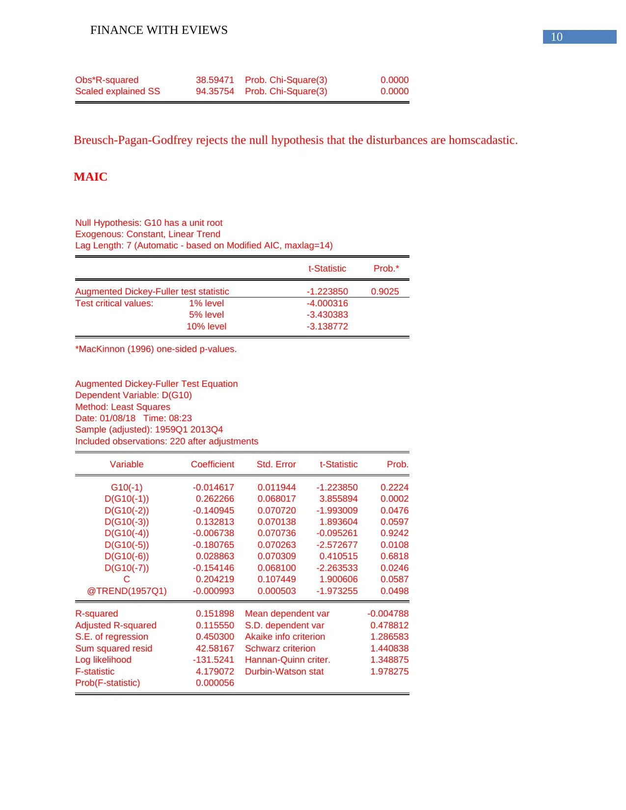
Breusch-Pagan-Godfrey rejects the null hypothesis that the disturbances are homscadastic.
MAIC
Null Hypothesis: G10 has a unit root
Exogenous: Constant, Linear Trend
Lag Length: 7 (Automatic - based on Modified AIC, maxlag=14)
t-Statistic Prob.*
Augmented Dickey-Fuller test statistic -1.223850 0.9025
Test critical values: 1% level -4.000316
5% level -3.430383
10% level -3.138772
*MacKinnon (1996) one-sided p-values.
Augmented Dickey-Fuller Test Equation
Dependent Variable: D(G10)
Method: Least Squares
Date: 01/08/18 Time: 08:23
Sample (adjusted): 1959Q1 2013Q4
Included observations: 220 after adjustments
Variable Coefficient Std. Error t-Statistic Prob.
G10(-1) -0.014617 0.011944 -1.223850 0.2224
D(G10(-1)) 0.262266 0.068017 3.855894 0.0002
D(G10(-2)) -0.140945 0.070720 -1.993009 0.0476
D(G10(-3)) 0.132813 0.070138 1.893604 0.0597
D(G10(-4)) -0.006738 0.070736 -0.095261 0.9242
D(G10(-5)) -0.180765 0.070263 -2.572677 0.0108
D(G10(-6)) 0.028863 0.070309 0.410515 0.6818
D(G10(-7)) -0.154146 0.068100 -2.263533 0.0246
C 0.204219 0.107449 1.900606 0.0587
@TREND(1957Q1) -0.000993 0.000503 -1.973255 0.0498
R-squared 0.151898 Mean dependent var -0.004788
Adjusted R-squared 0.115550 S.D. dependent var 0.478812
S.E. of regression 0.450300 Akaike info criterion 1.286583
Sum squared resid 42.58167 Schwarz criterion 1.440838
Log likelihood -131.5241 Hannan-Quinn criter. 1.348875
F-statistic 4.179072 Durbin-Watson stat 1.978275
Prob(F-statistic) 0.000056
FINANCE WITH EVIEWS
Obs*R-squared 38.59471 Prob. Chi-Square(3) 0.0000
Scaled explained SS 94.35754 Prob. Chi-Square(3) 0.0000
Breusch-Pagan-Godfrey rejects the null hypothesis that the disturbances are homscadastic.
MAIC
Null Hypothesis: G10 has a unit root
Exogenous: Constant, Linear Trend
Lag Length: 7 (Automatic - based on Modified AIC, maxlag=14)
t-Statistic Prob.*
Augmented Dickey-Fuller test statistic -1.223850 0.9025
Test critical values: 1% level -4.000316
5% level -3.430383
10% level -3.138772
*MacKinnon (1996) one-sided p-values.
Augmented Dickey-Fuller Test Equation
Dependent Variable: D(G10)
Method: Least Squares
Date: 01/08/18 Time: 08:23
Sample (adjusted): 1959Q1 2013Q4
Included observations: 220 after adjustments
Variable Coefficient Std. Error t-Statistic Prob.
G10(-1) -0.014617 0.011944 -1.223850 0.2224
D(G10(-1)) 0.262266 0.068017 3.855894 0.0002
D(G10(-2)) -0.140945 0.070720 -1.993009 0.0476
D(G10(-3)) 0.132813 0.070138 1.893604 0.0597
D(G10(-4)) -0.006738 0.070736 -0.095261 0.9242
D(G10(-5)) -0.180765 0.070263 -2.572677 0.0108
D(G10(-6)) 0.028863 0.070309 0.410515 0.6818
D(G10(-7)) -0.154146 0.068100 -2.263533 0.0246
C 0.204219 0.107449 1.900606 0.0587
@TREND(1957Q1) -0.000993 0.000503 -1.973255 0.0498
R-squared 0.151898 Mean dependent var -0.004788
Adjusted R-squared 0.115550 S.D. dependent var 0.478812
S.E. of regression 0.450300 Akaike info criterion 1.286583
Sum squared resid 42.58167 Schwarz criterion 1.440838
Log likelihood -131.5241 Hannan-Quinn criter. 1.348875
F-statistic 4.179072 Durbin-Watson stat 1.978275
Prob(F-statistic) 0.000056
11
FINANCE WITH EVIEWS
Dependent Variable: D(G10)
Method: Least Squares
Date: 01/08/18 Time: 08:25
Sample (adjusted): 1959Q1 2013Q4
Included observations: 220 after adjustments
Variable Coefficient Std. Error t-Statistic Prob.
C 0.204219 0.107449 1.900606 0.0587
G10(-1) -0.014617 0.011944 -1.223850 0.2224
D(G10(-1)) 0.262266 0.068017 3.855894 0.0002
D(G10(-2)) -0.140945 0.070720 -1.993009 0.0476
D(G10(-3)) 0.132813 0.070138 1.893604 0.0597
D(G10(-4)) -0.006738 0.070736 -0.095261 0.9242
D(G10(-5)) -0.180765 0.070263 -2.572677 0.0108
D(G10(-6)) 0.028863 0.070309 0.410515 0.6818
D(G10(-7)) -0.154146 0.068100 -2.263533 0.0246
@TREND -0.000993 0.000503 -1.973255 0.0498
R-squared 0.151898 Mean dependent var -0.004788
Adjusted R-squared 0.115550 S.D. dependent var 0.478812
S.E. of regression 0.450300 Akaike info criterion 1.286583
Sum squared resid 42.58167 Schwarz criterion 1.440838
Log likelihood -131.5241 Hannan-Quinn criter. 1.348875
F-statistic 4.179072 Durbin-Watson stat 1.978275
Prob(F-statistic) 0.000056
Breusch-Godfrey Serial Correlation LM Test:
F-statistic 0.557354 Prob. F(2,208) 0.5736
Obs*R-squared 1.172733 Prob. Chi-Square(2) 0.5563
Heteroskedasticity Test: Breusch-Pagan-Godfrey
F-statistic 6.438922 Prob. F(9,210) 0.0000
Obs*R-squared 47.57996 Prob. Chi-Square(9) 0.0000
Scaled explained SS 98.80355 Prob. Chi-Square(9) 0.0000
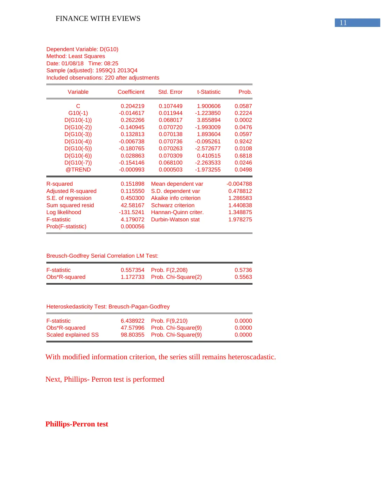
With modified information criterion, the series still remains heteroscadastic.
Next, Phillips- Perron test is performed
Phillips-Perron test
FINANCE WITH EVIEWS
Dependent Variable: D(G10)
Method: Least Squares
Date: 01/08/18 Time: 08:25
Sample (adjusted): 1959Q1 2013Q4
Included observations: 220 after adjustments
Variable Coefficient Std. Error t-Statistic Prob.
C 0.204219 0.107449 1.900606 0.0587
G10(-1) -0.014617 0.011944 -1.223850 0.2224
D(G10(-1)) 0.262266 0.068017 3.855894 0.0002
D(G10(-2)) -0.140945 0.070720 -1.993009 0.0476
D(G10(-3)) 0.132813 0.070138 1.893604 0.0597
D(G10(-4)) -0.006738 0.070736 -0.095261 0.9242
D(G10(-5)) -0.180765 0.070263 -2.572677 0.0108
D(G10(-6)) 0.028863 0.070309 0.410515 0.6818
D(G10(-7)) -0.154146 0.068100 -2.263533 0.0246
@TREND -0.000993 0.000503 -1.973255 0.0498
R-squared 0.151898 Mean dependent var -0.004788
Adjusted R-squared 0.115550 S.D. dependent var 0.478812
S.E. of regression 0.450300 Akaike info criterion 1.286583
Sum squared resid 42.58167 Schwarz criterion 1.440838
Log likelihood -131.5241 Hannan-Quinn criter. 1.348875
F-statistic 4.179072 Durbin-Watson stat 1.978275
Prob(F-statistic) 0.000056
Breusch-Godfrey Serial Correlation LM Test:
F-statistic 0.557354 Prob. F(2,208) 0.5736
Obs*R-squared 1.172733 Prob. Chi-Square(2) 0.5563
Heteroskedasticity Test: Breusch-Pagan-Godfrey
F-statistic 6.438922 Prob. F(9,210) 0.0000
Obs*R-squared 47.57996 Prob. Chi-Square(9) 0.0000
Scaled explained SS 98.80355 Prob. Chi-Square(9) 0.0000
With modified information criterion, the series still remains heteroscadastic.
Next, Phillips- Perron test is performed
Phillips-Perron test
⊘ This is a preview!⊘
Do you want full access?
Subscribe today to unlock all pages.
Trusted by 1+ million students worldwide
1 out of 31
Related Documents


Your All-in-One AI-Powered Toolkit for Academic Success.
+13062052269
info@desklib.com
Available 24*7 on WhatsApp / Email
![[object Object]](/_next/static/media/star-bottom.7253800d.svg)
Unlock your academic potential
Copyright © 2020–2026 A2Z Services. All Rights Reserved. Developed and managed by ZUCOL.