Excel Pivot Table Analysis on Lodgement Methods Dataset

The assignment involves analyzing two datasets concerning lodgement methods using Excel's data analysis capabilities. Students create pivot tables to summarize data by different categories such as age group and income. They use these tables to generate 3D pie charts for visual representation of data distribution across lodgement methods. The task also includes calculating confidence intervals, performing chi-square tests for categorical variables, and examining the relationship between total income and deduction amounts through regression analysis. Students are required to employ Excel's statistical functions to derive insights from the provided datasets effectively.

Lodgement Method: Dataset 1
To answer this question, at first a pivot table is inserted in excel by choosing the whole
data as the table range and then selecting lodgement method under rows and values. This results
in the table 2 in the answer file. Inserting a pivot chart and selecting 3d pie chart gives figure 1.
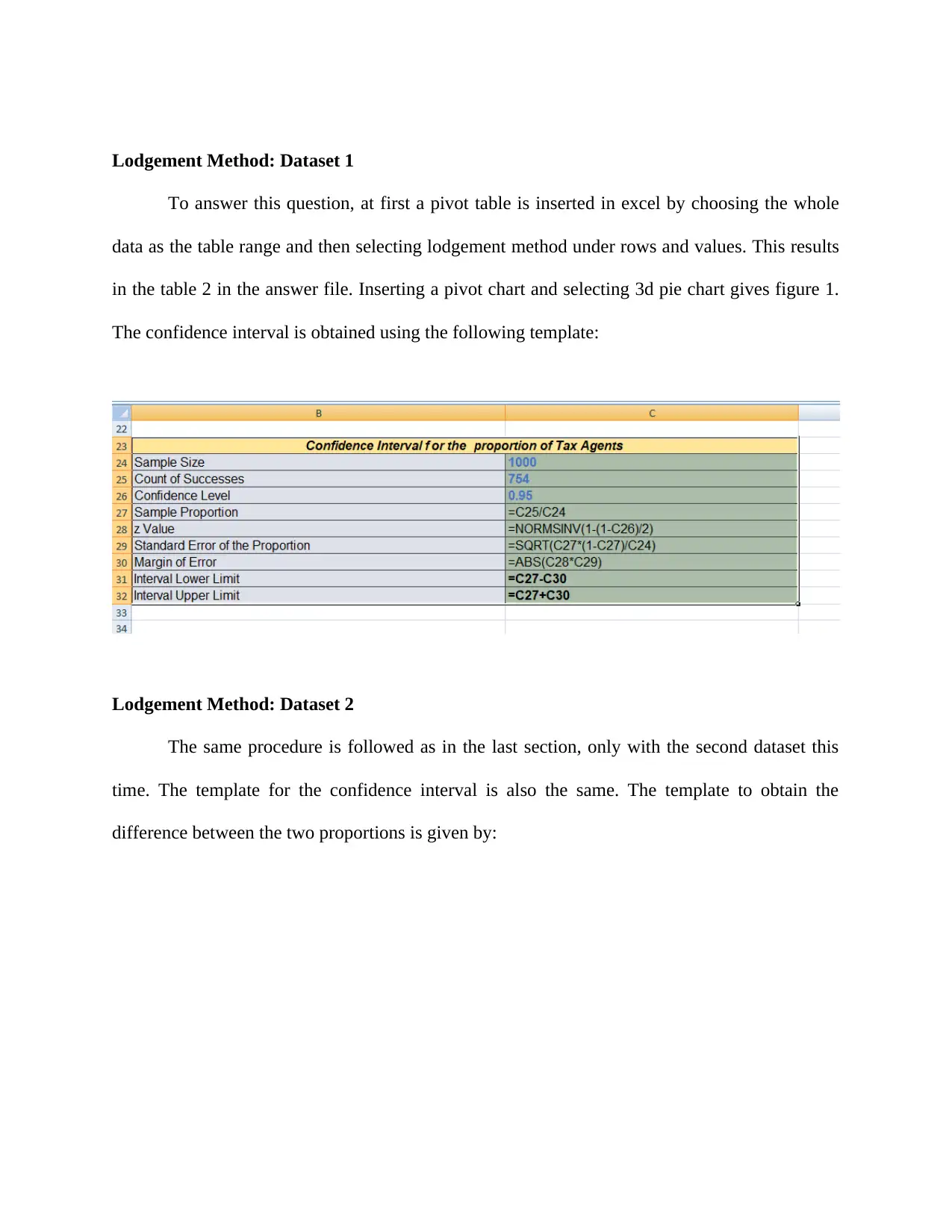
The confidence interval is obtained using the following template:
Lodgement Method: Dataset 2
The same procedure is followed as in the last section, only with the second dataset this
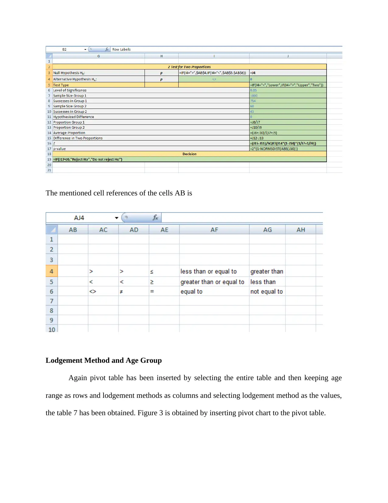
time. The template for the confidence interval is also the same. The template to obtain the
difference between the two proportions is given by:

The mentioned cell references of the cells AB is
Lodgement Method and Age Group
Again pivot table has been inserted by selecting the entire table and then keeping age
range as rows and lodgement methods as columns and selecting lodgement method as the values,
the table 7 has been obtained. Figure 3 is obtained by inserting pivot chart to the pivot table.

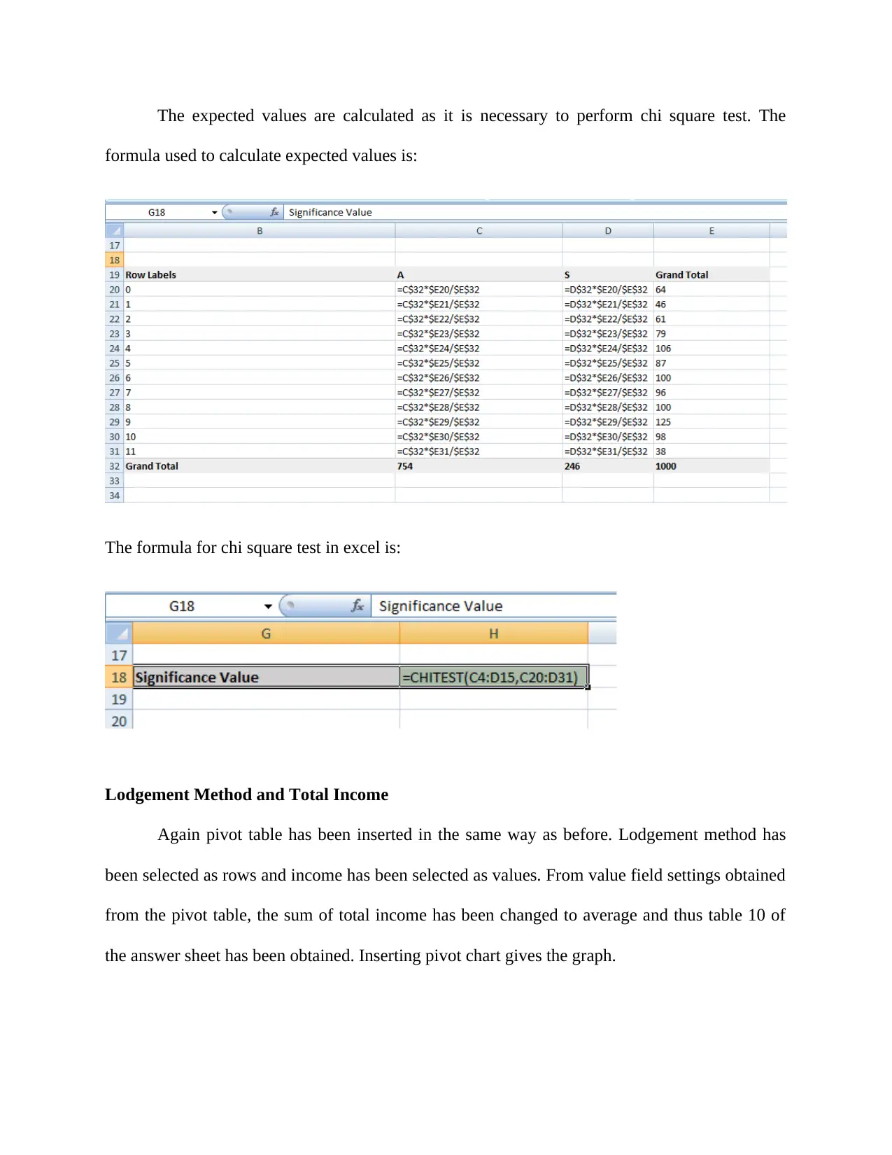
The expected values are calculated as it is necessary to perform chi square test. The
formula used to calculate expected values is:
The formula for chi square test in excel is:
Lodgement Method and Total Income
Again pivot table has been inserted in the same way as before. Lodgement method has
been selected as rows and income has been selected as values. From value field settings obtained
from the pivot table, the sum of total income has been changed to average and thus table 10 of
the answer sheet has been obtained. Inserting pivot chart gives the graph.

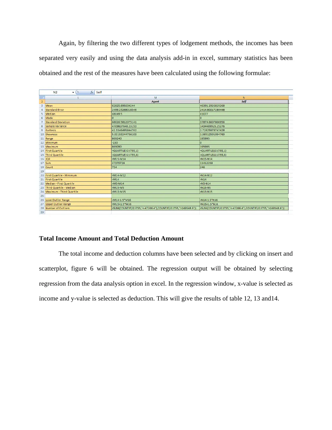
Again, by filtering the two different types of lodgement methods, the incomes has been
separated very easily and using the data analysis add-in in excel, summary statistics has been
obtained and the rest of the measures have been calculated using the following formulae:
Total Income Amount and Total Deduction Amount
The total income and deduction columns have been selected and by clicking on insert and
scatterplot, figure 6 will be obtained. The regression output will be obtained by selecting
regression from the data analysis option in excel. In the regression window, x-value is selected as
income and y-value is selected as deduction. This will give the results of table 12, 13 and14.