Excise Duty, Market Structures, and the Economics of Local Mergers
VerifiedAdded on 2023/06/12
|16
|2689
|496
Homework Assignment
AI Summary
This assignment provides a detailed analysis of several key economic concepts. It begins by examining the impact of excise duty on goods like cigarettes, focusing on price elasticity of demand and its implications for consumers and government revenue. The assignment then contrasts monopolistic and oligopolistic market structures, detailing their characteristics, price and output determination, and examples. Finally, it explores the economic rationale behind local council mergers in Australia, using cost curve models to illustrate potential efficiencies and limitations. Desklib offers a wealth of similar assignments and study resources for students.
Contents
Question 1...................................................................................................................................................1
Question 2...................................................................................................................................................2
a) Fixed and Variable Costs..................................................................................................................2
b) Differences between Monopolistic and Oligopolistic Market Structures........................................3
Price and Output determination in a Monopolistic Competition..............................................................5
Short Run Equilibrium.........................................................................................................................5
Long Run Equilibrium.........................................................................................................................7
Question 3.................................................................................................................................................11
Paraphrase This Document
Need a fresh take? Get an instant paraphrase of this document with our AI Paraphraser
Question 1
a) There is an excise duty (tax rate) is as follows Australian Taxation Office, (2018)
Tax Rate Retail Price Base Price
Upto Jan 2018 0.6898 30 17.7535
Since March 2018 0.71046 30 21.3138
Price Elasticity refers to the degree to which the demand a good is price sensitive. i.e. if a small
increase in the price, reduces the demand disproportionately (greater than 1), then the demand for
the god is highly price elastic. Similarly, if the demand for the good is relatively unaffected, then
the price elasticity is low. (Less than 1) (Mankiw, 2008)
It is measured as:
EDP = Proportionate change in demand/ proportionate change in per unit price.
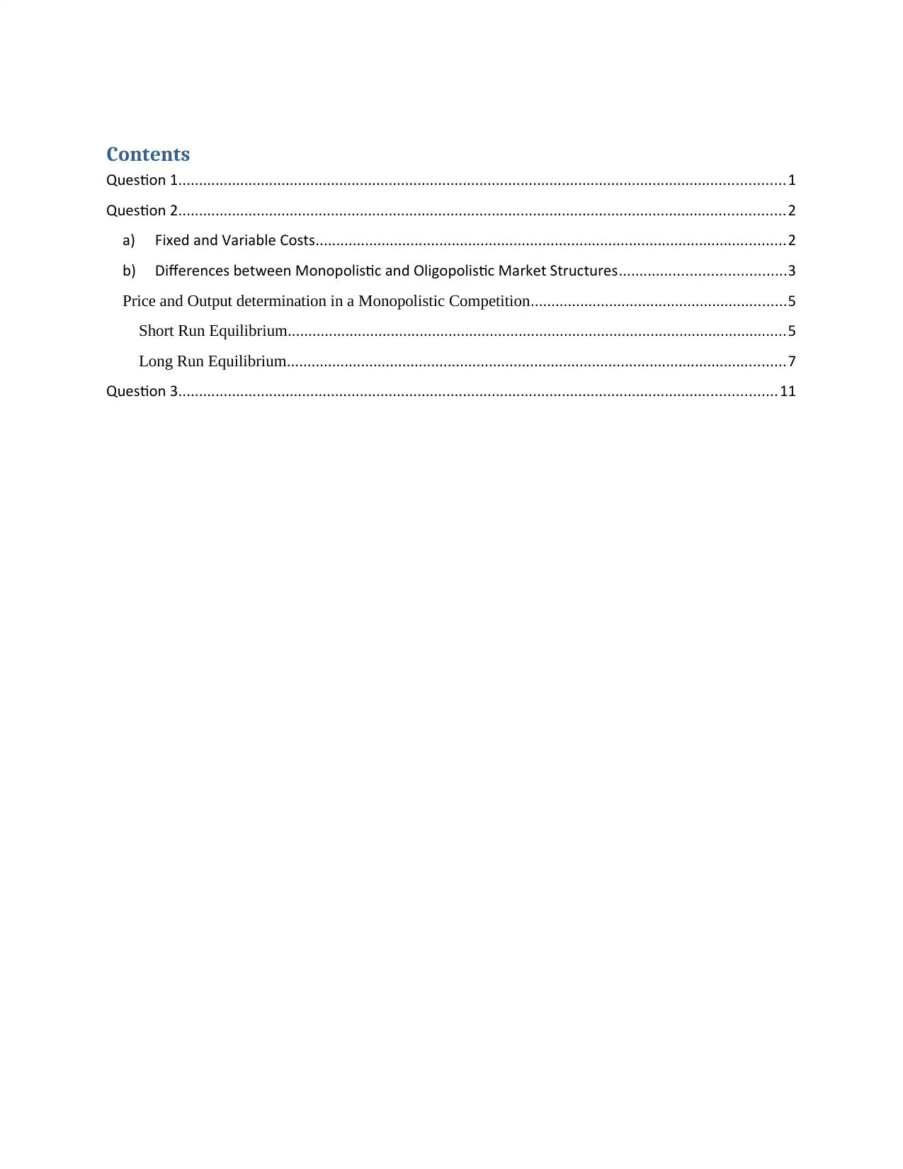
Figure 1 Price Elasticity of Demand
Source: (Samuelson & Nordhaus, 2006)
In the diagram above, as the price drops from P1 to P2, the demand (and consequently output)
moves from Q1 to Q3. The ratio of (P2-P1)/(Q2-Q1) is the elasticity of demand. The reverse effect
a) There is an excise duty (tax rate) is as follows Australian Taxation Office, (2018)
Tax Rate Retail Price Base Price
Upto Jan 2018 0.6898 30 17.7535
Since March 2018 0.71046 30 21.3138
Price Elasticity refers to the degree to which the demand a good is price sensitive. i.e. if a small
increase in the price, reduces the demand disproportionately (greater than 1), then the demand for
the god is highly price elastic. Similarly, if the demand for the good is relatively unaffected, then
the price elasticity is low. (Less than 1) (Mankiw, 2008)
It is measured as:
EDP = Proportionate change in demand/ proportionate change in per unit price.
Figure 1 Price Elasticity of Demand
Source: (Samuelson & Nordhaus, 2006)
In the diagram above, as the price drops from P1 to P2, the demand (and consequently output)
moves from Q1 to Q3. The ratio of (P2-P1)/(Q2-Q1) is the elasticity of demand. The reverse effect
is seen as price increases from P1 to P3. Output falls fromQ1 and Q2 and hence the (P3- P1/ Q1- Q3)
elasticity will be negative.
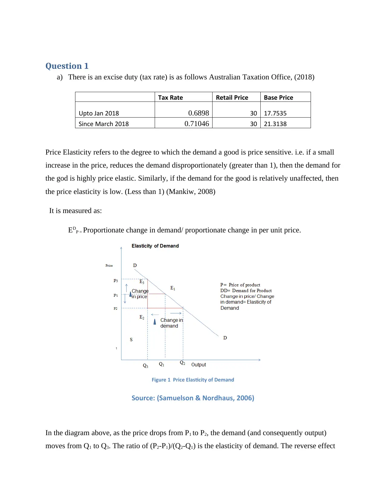
Figure 2 Various kinds Price Elasticity of Demand
Source: (Chauhan 2009)
According to international research, generally, the elasticity of demand for cigarettes in Western
Countries is less approximately -0.4. (Tobacco in Australia, 2018)Thus, the Price Elasticity of
demand for cigarettes is low (Panel 2 of Figure2). Hence, an increase in the tax would not reduce
the demand in the same proportion. (Mankiw, 2008) Tobacco consumption has decreased
significantly in Australia and taxation has played a role in this transformation. (Australian
Bureau of Statistics, 2013)
elasticity will be negative.
Figure 2 Various kinds Price Elasticity of Demand
Source: (Chauhan 2009)
According to international research, generally, the elasticity of demand for cigarettes in Western
Countries is less approximately -0.4. (Tobacco in Australia, 2018)Thus, the Price Elasticity of
demand for cigarettes is low (Panel 2 of Figure2). Hence, an increase in the tax would not reduce
the demand in the same proportion. (Mankiw, 2008) Tobacco consumption has decreased
significantly in Australia and taxation has played a role in this transformation. (Australian
Bureau of Statistics, 2013)
⊘ This is a preview!⊘
Do you want full access?
Subscribe today to unlock all pages.
Trusted by 1+ million students worldwide
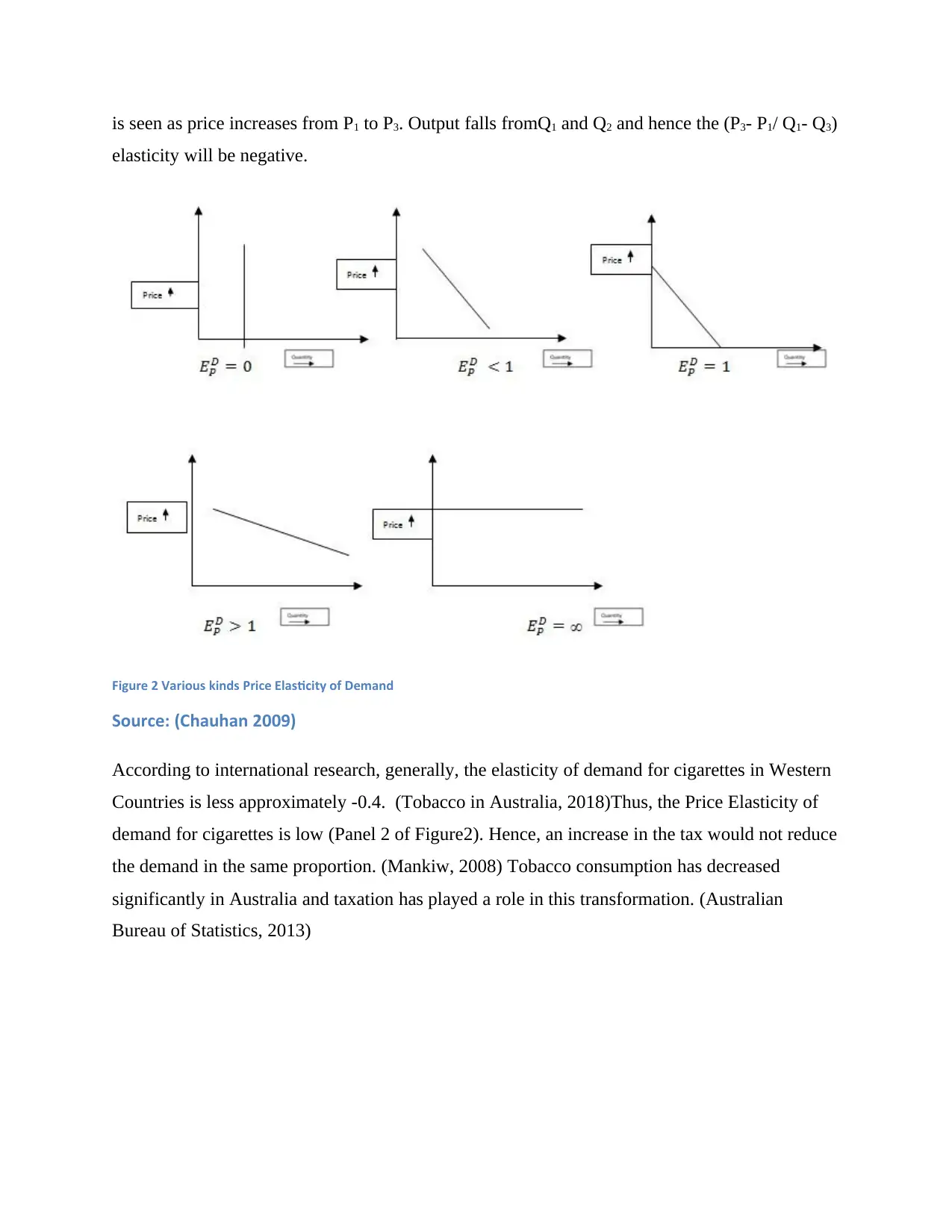
Figure 3 The Effect of Taxes on Tobacco Based Products (Example: Cigarettes)
Since, the demand is not expected to reduce to a great extent, if the price changes considerably,
the seller can afford to pass it on to the consumer, Thus, the consumer will have to pay a higher
price of the cigarette. The implication of this is that the consumer will either be forced to pay
more or decrease consumption. The benefit of this is received in the form of greater public
health. Additionally, given that the demand for cigarettes is highly inelastic and the demand is
not expected to shrink much, there is the possibility of additional revenue to the government.
(Mankiw, 2008)
Question 2
a) Fixed and Variable Costs
b) Marginal Costs is calculated as the cost of the “last unit produced i.e Current Total Costs
– Previous Total Costs for every level of output. (Chauhan, 2009)
Paraphrase This Document
Need a fresh take? Get an instant paraphrase of this document with our AI Paraphraser
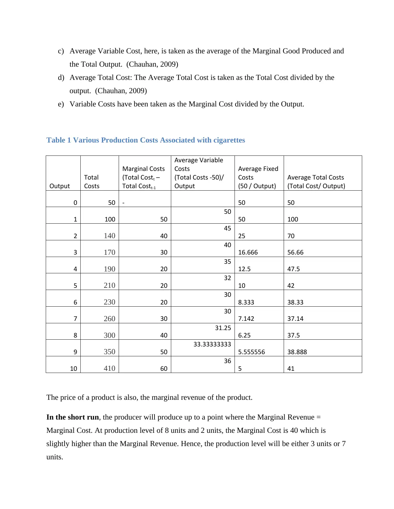
c) Average Variable Cost, here, is taken as the average of the Marginal Good Produced and
the Total Output. (Chauhan, 2009)
d) Average Total Cost: The Average Total Cost is taken as the Total Cost divided by the
output. (Chauhan, 2009)
e) Variable Costs have been taken as the Marginal Cost divided by the Output.
Table 1 Various Production Costs Associated with cigarettes
Output
Total
Costs
Marginal Costs
(Total Costt –
Total Costt-1
Average Variable
Costs
(Total Costs -50)/
Output
Average Fixed
Costs
(50 / Output)
Average Total Costs
(Total Cost/ Output)
0 50 - 50 50
1 100 50
50
50 100
2 140 40
45
25 70
3 170 30
40
16.666 56.66
4 190 20
35
12.5 47.5
5 210 20
32
10 42
6 230 20
30
8.333 38.33
7 260 30
30
7.142 37.14
8 300 40
31.25
6.25 37.5
9 350 50
33.33333333
5.555556 38.888
10 410 60
36
5 41
The price of a product is also, the marginal revenue of the product.
In the short run, the producer will produce up to a point where the Marginal Revenue =
Marginal Cost. At production level of 8 units and 2 units, the Marginal Cost is 40 which is
slightly higher than the Marginal Revenue. Hence, the production level will be either 3 units or 7
units.
At the production level of 3 units, the Total Revenue of the good will be :
Total revenue = Price X Output
= $(35 X3)
= $105.
However, at this level, the total costs are at $170.
Hence, the Profits are
Profits = Total Revenue – Total Costs
= $170- $105
= - $65.
There is a net loss of $ 65 at this level.
At production level of 7 units, the Total Revenue is
Total revenue = Price X Output
Total revenue = $35 X 7
= $245
At this level , the Profits are
Profits = Total Revenue – Total Costs
= $245- $260
= - $15
Hence, the seller will stop production at 7 units since the seller is trying to minimize losses.
In the long run, the producer will produce where the average cost (long run average cost) is the
lowest. This is at output level 8 and 7. Since, the Marginal costs is lowest at 7, the producer will
still produce 7 units.
Total revenue = Price X Output
= $(35 X3)
= $105.
However, at this level, the total costs are at $170.
Hence, the Profits are
Profits = Total Revenue – Total Costs
= $170- $105
= - $65.
There is a net loss of $ 65 at this level.
At production level of 7 units, the Total Revenue is
Total revenue = Price X Output
Total revenue = $35 X 7
= $245
At this level , the Profits are
Profits = Total Revenue – Total Costs
= $245- $260
= - $15
Hence, the seller will stop production at 7 units since the seller is trying to minimize losses.
In the long run, the producer will produce where the average cost (long run average cost) is the
lowest. This is at output level 8 and 7. Since, the Marginal costs is lowest at 7, the producer will
still produce 7 units.
⊘ This is a preview!⊘
Do you want full access?
Subscribe today to unlock all pages.
Trusted by 1+ million students worldwide
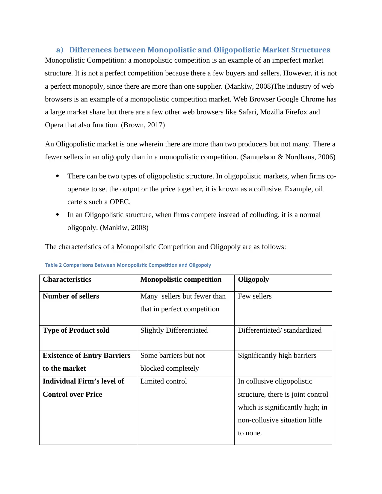
a) Differences between Monopolistic and Oligopolistic Market Structures
Monopolistic Competition: a monopolistic competition is an example of an imperfect market
structure. It is not a perfect competition because there a few buyers and sellers. However, it is not
a perfect monopoly, since there are more than one supplier. (Mankiw, 2008)The industry of web
browsers is an example of a monopolistic competition market. Web Browser Google Chrome has
a large market share but there are a few other web browsers like Safari, Mozilla Firefox and
Opera that also function. (Brown, 2017)
An Oligopolistic market is one wherein there are more than two producers but not many. There a
fewer sellers in an oligopoly than in a monopolistic competition. (Samuelson & Nordhaus, 2006)
There can be two types of oligopolistic structure. In oligopolistic markets, when firms co-
operate to set the output or the price together, it is known as a collusive. Example, oil
cartels such a OPEC.
In an Oligopolistic structure, when firms compete instead of colluding, it is a normal
oligopoly. (Mankiw, 2008)
The characteristics of a Monopolistic Competition and Oligopoly are as follows:
Table 2 Comparisons Between Monopolistic Competition and Oligopoly
Characteristics Monopolistic competition Oligopoly
Number of sellers Many sellers but fewer than
that in perfect competition
Few sellers
Type of Product sold Slightly Differentiated Differentiated/ standardized
Existence of Entry Barriers
to the market
Some barriers but not
blocked completely
Significantly high barriers
Individual Firm’s level of
Control over Price
Limited control In collusive oligopolistic
structure, there is joint control
which is significantly high; in
non-collusive situation little
to none.
Paraphrase This Document
Need a fresh take? Get an instant paraphrase of this document with our AI Paraphraser
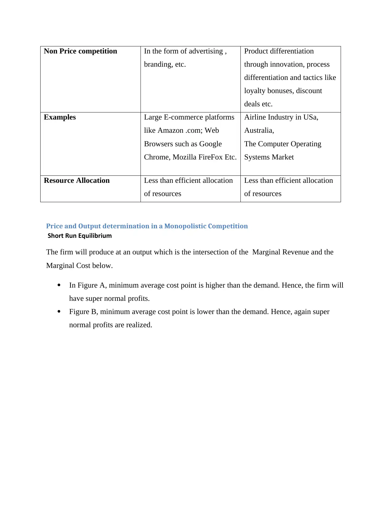
Non Price competition In the form of advertising ,
branding, etc.
Product differentiation
through innovation, process
differentiation and tactics like
loyalty bonuses, discount
deals etc.
Examples Large E-commerce platforms
like Amazon .com; Web
Browsers such as Google
Chrome, Mozilla FireFox Etc.
Airline Industry in USa,
Australia,
The Computer Operating
Systems Market
Resource Allocation Less than efficient allocation
of resources
Less than efficient allocation
of resources
Price and Output determination in a Monopolistic Competition
Short Run Equilibrium
The firm will produce at an output which is the intersection of the Marginal Revenue and the
Marginal Cost below.
In Figure A, minimum average cost point is higher than the demand. Hence, the firm will
have super normal profits.
Figure B, minimum average cost point is lower than the demand. Hence, again super
normal profits are realized.
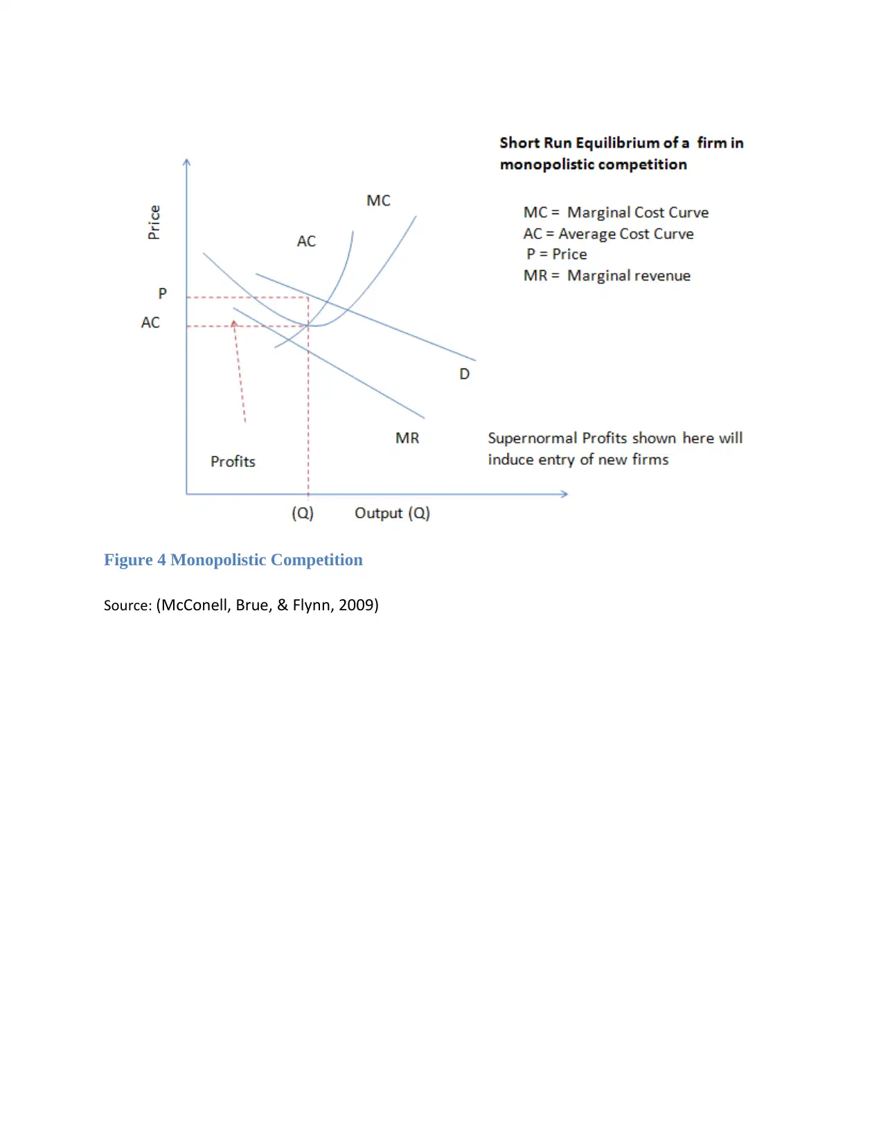
Figure 4 Monopolistic Competition
Source: (McConell, Brue, & Flynn, 2009)
Source: (McConell, Brue, & Flynn, 2009)
⊘ This is a preview!⊘
Do you want full access?
Subscribe today to unlock all pages.
Trusted by 1+ million students worldwide
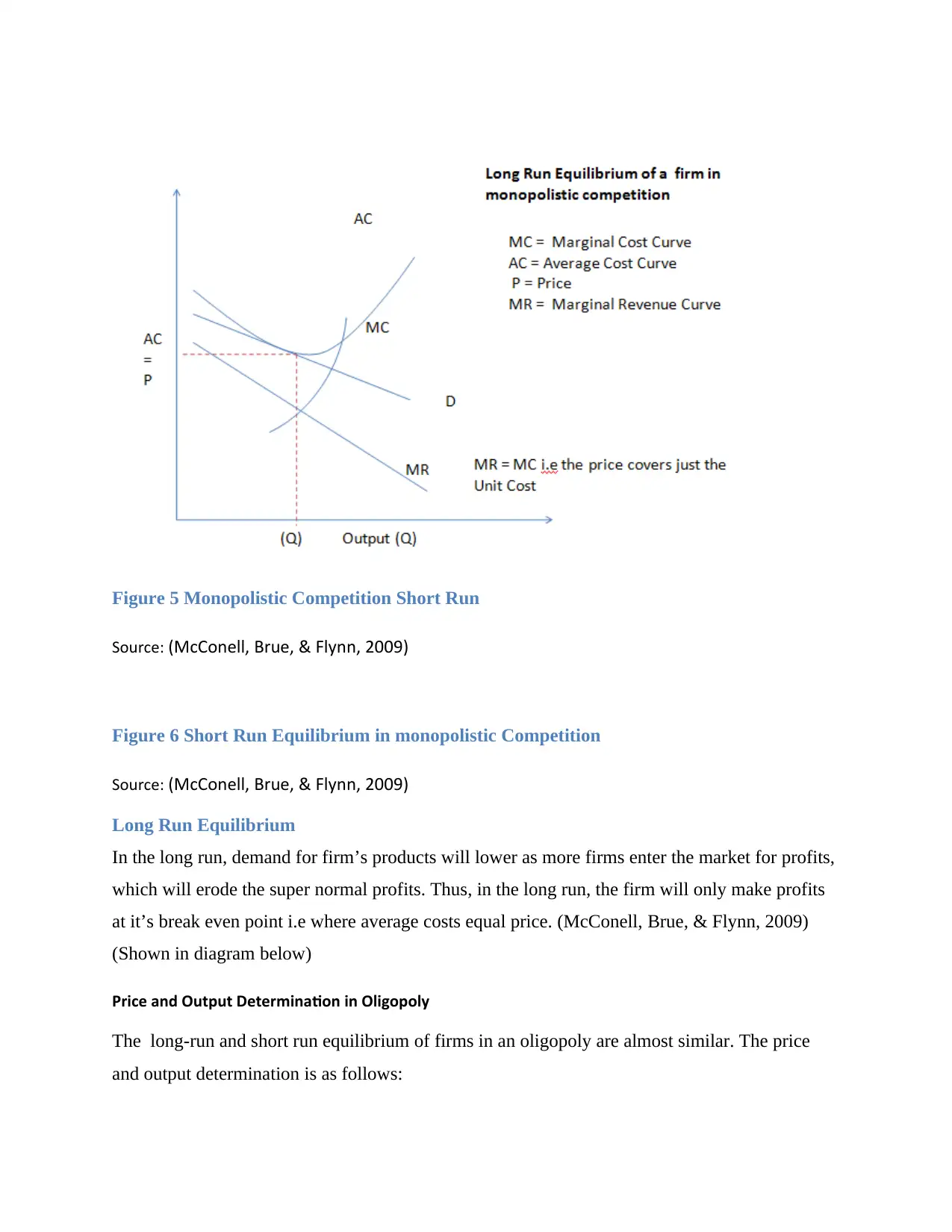
Figure 5 Monopolistic Competition Short Run
Source: (McConell, Brue, & Flynn, 2009)
Figure 6 Short Run Equilibrium in monopolistic Competition
Source: (McConell, Brue, & Flynn, 2009)
Long Run Equilibrium
In the long run, demand for firm’s products will lower as more firms enter the market for profits,
which will erode the super normal profits. Thus, in the long run, the firm will only make profits
at it’s break even point i.e where average costs equal price. (McConell, Brue, & Flynn, 2009)
(Shown in diagram below)
Price and Output Determination in Oligopoly
The long-run and short run equilibrium of firms in an oligopoly are almost similar. The price
and output determination is as follows:
Source: (McConell, Brue, & Flynn, 2009)
Figure 6 Short Run Equilibrium in monopolistic Competition
Source: (McConell, Brue, & Flynn, 2009)
Long Run Equilibrium
In the long run, demand for firm’s products will lower as more firms enter the market for profits,
which will erode the super normal profits. Thus, in the long run, the firm will only make profits
at it’s break even point i.e where average costs equal price. (McConell, Brue, & Flynn, 2009)
(Shown in diagram below)
Price and Output Determination in Oligopoly
The long-run and short run equilibrium of firms in an oligopoly are almost similar. The price
and output determination is as follows:
Paraphrase This Document
Need a fresh take? Get an instant paraphrase of this document with our AI Paraphraser
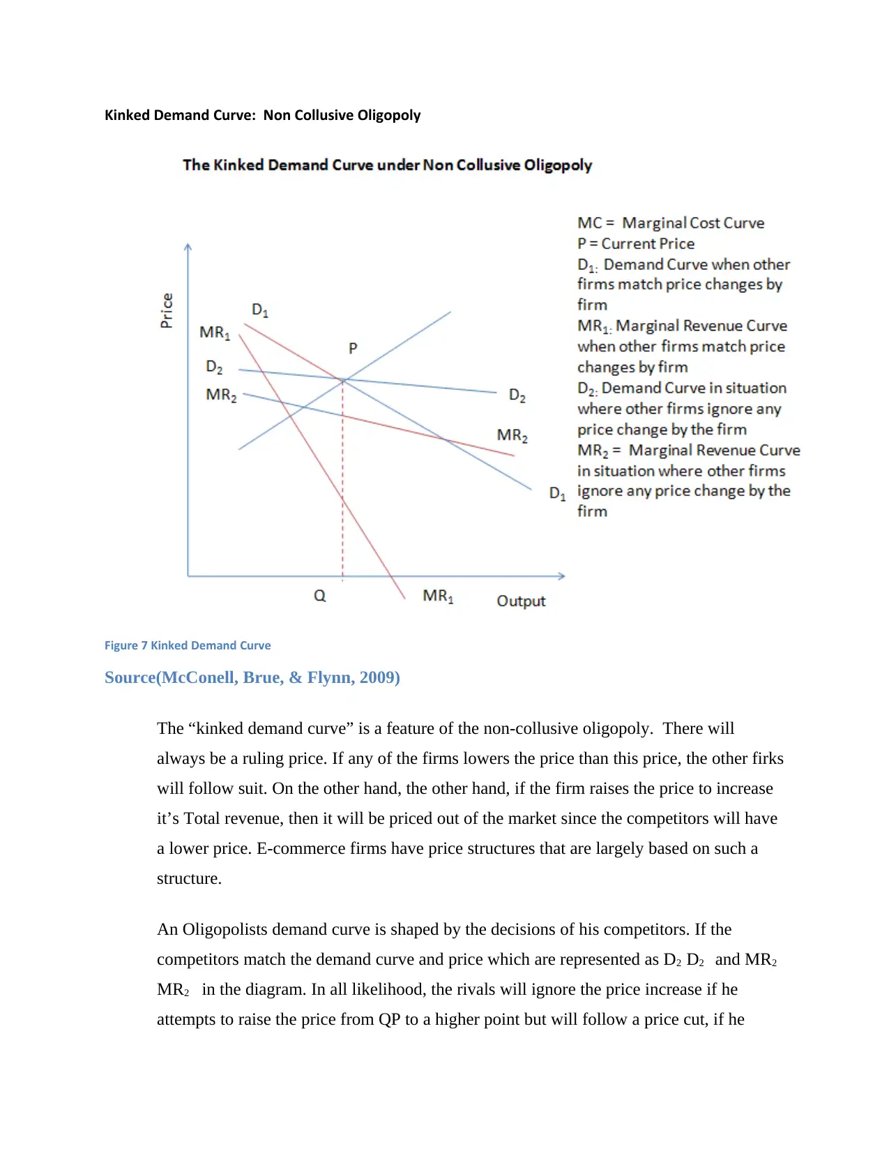
Kinked Demand Curve: Non Collusive Oligopoly
Figure 7 Kinked Demand Curve
Source(McConell, Brue, & Flynn, 2009)
The “kinked demand curve” is a feature of the non-collusive oligopoly. There will
always be a ruling price. If any of the firms lowers the price than this price, the other firks
will follow suit. On the other hand, the other hand, if the firm raises the price to increase
it’s Total revenue, then it will be priced out of the market since the competitors will have
a lower price. E-commerce firms have price structures that are largely based on such a
structure.
An Oligopolists demand curve is shaped by the decisions of his competitors. If the
competitors match the demand curve and price which are represented as D2 D2 and MR2
MR2 in the diagram. In all likelihood, the rivals will ignore the price increase if he
attempts to raise the price from QP to a higher point but will follow a price cut, if he
lowers the price. Thus, the demand curve is kinked i.e D2 P D1 and the Marginal
Revenue is broken at MR2 MR1
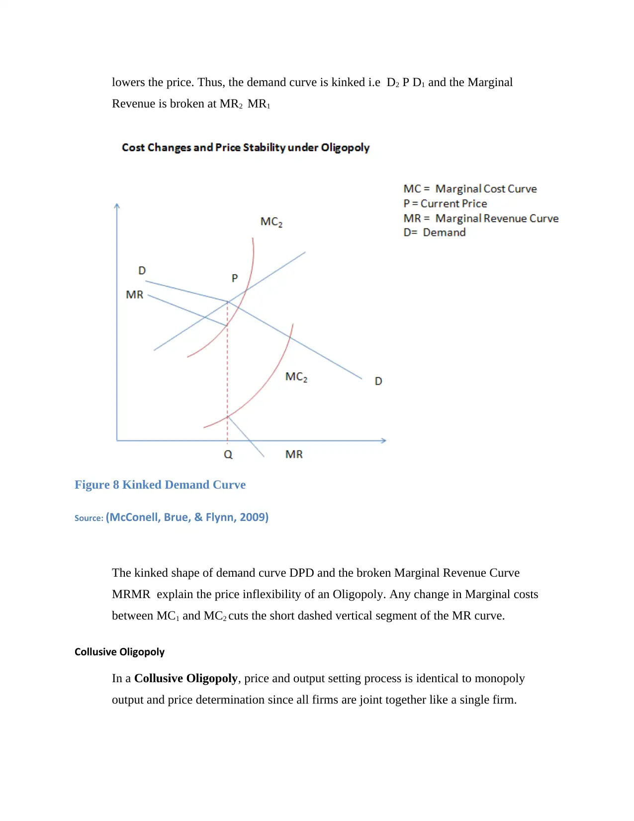
Figure 8 Kinked Demand Curve
Source: (McConell, Brue, & Flynn, 2009)
The kinked shape of demand curve DPD and the broken Marginal Revenue Curve
MRMR explain the price inflexibility of an Oligopoly. Any change in Marginal costs
between MC1 and MC2 cuts the short dashed vertical segment of the MR curve.
Collusive Oligopoly
In a Collusive Oligopoly, price and output setting process is identical to monopoly
output and price determination since all firms are joint together like a single firm.
Revenue is broken at MR2 MR1
Figure 8 Kinked Demand Curve
Source: (McConell, Brue, & Flynn, 2009)
The kinked shape of demand curve DPD and the broken Marginal Revenue Curve
MRMR explain the price inflexibility of an Oligopoly. Any change in Marginal costs
between MC1 and MC2 cuts the short dashed vertical segment of the MR curve.
Collusive Oligopoly
In a Collusive Oligopoly, price and output setting process is identical to monopoly
output and price determination since all firms are joint together like a single firm.
⊘ This is a preview!⊘
Do you want full access?
Subscribe today to unlock all pages.
Trusted by 1+ million students worldwide
1 out of 16
Related Documents


Your All-in-One AI-Powered Toolkit for Academic Success.
+13062052269
info@desklib.com
Available 24*7 on WhatsApp / Email
![[object Object]](/_next/static/media/star-bottom.7253800d.svg)
Unlock your academic potential
Copyright © 2020–2026 A2Z Services. All Rights Reserved. Developed and managed by ZUCOL.