Analysis of Order Data: Financial Statistics Report for Executives

This report provides a financial statistical analysis of order data, focusing on a sample of 60 orders from a larger dataset of 2002 orders. The analysis includes frequency tables, confidence intervals, hypothesis testing, and correlation/regression analysis to provide insights into sales, shipping costs, customer segments, and order priorities. Key findings include the identification of high-priority orders and the East/West regions as areas for increased sales focus. The report also examines the relationship between order quantity and sales, revealing a positive correlation. The limitations of the report include the small sample size which might impact the results. Overall, the report aims to provide actionable insights for executive decision-making, including the importance of focusing on critical priority orders and East and West regions for increasing sales.

Financial Statistics

Executive summary
The report is developed in order to analyze the data of orders of the products and present to
the executive. A sample size of 60 orders has been chosen from the data of 2002 orders. The
data related to shipping costs, order priority, ship mode, consumer segment, days to ship and
shipping region has been analyzed. The tabular techniques, graphical techniques and
summary statistics are used to analyze the data. The mean, median, mode, standard deviation,
range and coefficient of variation of order quantity, sales and shipping cost have been
identified. It has been found that most of the sales range from $0 to $1000. The confidence
interval mean of sales for orders of home office customers is higher in contrast to that of the
mean of 2002 orders. There is a high difference among the confidence intervals of sales for
home office customers of selected sample and the whole data set. The hypothesis testing
shows that it is important to focus on critical priority orders and low priority orders for
increasing the profits and on east and west regions for increasing sales. The limitations of this
report are that the sample selected for the analysis is small which can affect the actual results
of the data of the orders.

Table of Contents
Introduction................................................................................................................................4
Data summary............................................................................................................................4
Confidence Intervals..................................................................................................................9
Hypothesis testing....................................................................................................................10
Correlation and regression.......................................................................................................11
Conclusion................................................................................................................................12
References................................................................................................................................13
Appendix..................................................................................................................................14

Introduction
The purpose of the report is to discuss and analyze 2002 orders data in order to present to the
executive. The analysis of the orders data has been performed in order to analyze the different
variables that are customers segment, order quantity, sales, region, and order priority. In the
report, a sample of 60 orders is selected. The frequency tables, confidence intervals,
hypothesis testing and correlation and regression are included in this report for analyzing the
data of orders. This will help in providing the insights to the executive related orders and will
provide the ability to make the tight decision in the future.Graphical and summary statistical
techniques are used in order to describe the orders using the variables. The selected sample
size is used from the data of 2002 orders in order to perform the analysis (refer table 1).The
reports will help in providing with the information related to the relationship among the
different variables.
Data summary
From the excel sheet consisting of the data of 2002 orders, a sample size of 60 orders has
been selected (Refer table 1). Graphical and summary statistical techniques are used in order
to describe the orders using the variables.
The frequency is considered as a measure of occurrences of a specific number of elements in
a set of data(Rumsey, 2016). A frequency table is considered as a method of arranging raw
data in compressed form, through presenting the data occurrence along with their
frequencies(Salkind, 2010). The frequency table for the sample data has been developed for
the different variables (refer table 2.).
It has been found with the help of the frequency table for order priority variable that high
order priority is highest in comparison to the other orders (refer Fig. 1). Hence, it is important

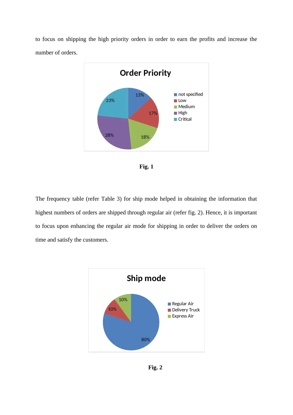
to focus on shipping the high priority orders in order to earn the profits and increase the
number of orders.
13%
17%
18%28%
23%
Order Priority
not specified
Low
Medium
High
Critical
Fig. 1
The frequency table (refer Table 3) for ship mode helped in obtaining the information that
highest numbers of orders are shipped through regular air (refer fig. 2). Hence, it is important
to focus upon enhancing the regular air mode for shipping in order to deliver the orders on
time and satisfy the customers.
80%
10%
10%
Ship mode
Regular Air
Delivery Truck
Express Air
Fig. 2

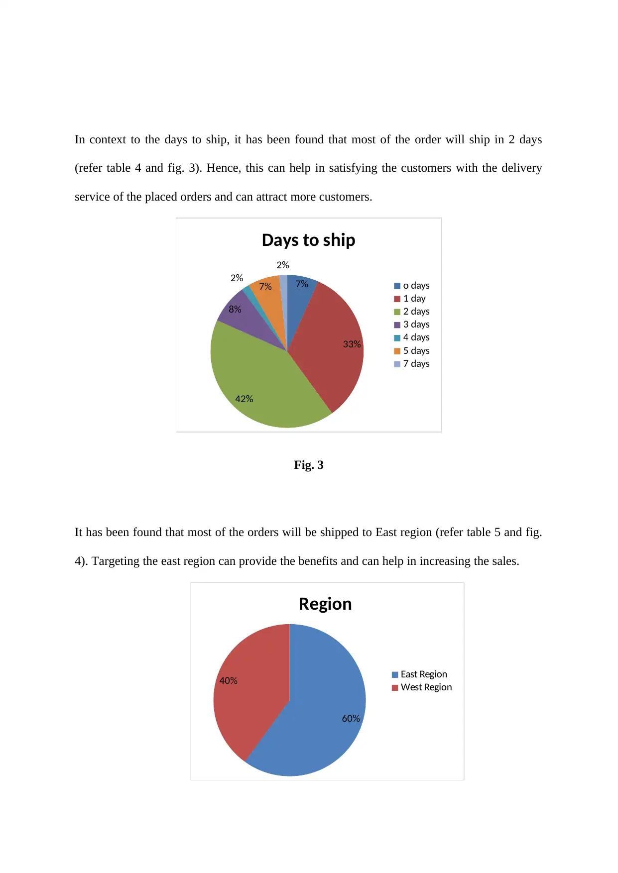
In context to the days to ship, it has been found that most of the order will ship in 2 days
(refer table 4 and fig. 3). Hence, this can help in satisfying the customers with the delivery
service of the placed orders and can attract more customers.
7%
33%
42%
8%
2% 7%
2%
Days to ship
o days
1 day
2 days
3 days
4 days
5 days
7 days
Fig. 3
It has been found that most of the orders will be shipped to East region (refer table 5 and fig.
4). Targeting the east region can provide the benefits and can help in increasing the sales.
60%
40%
Region
East Region
West Region

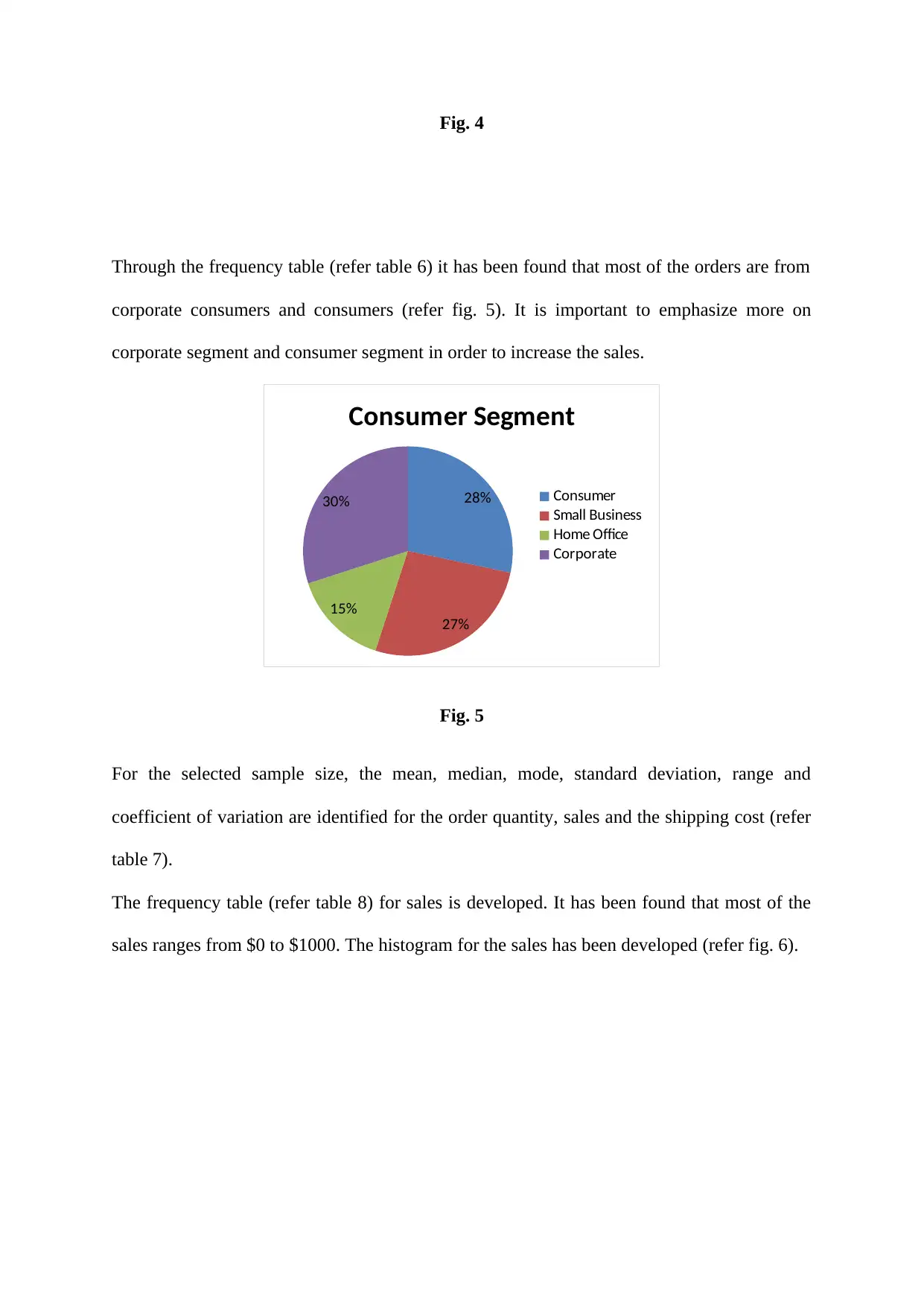
Fig. 4
Through the frequency table (refer table 6) it has been found that most of the orders are from
corporate consumers and consumers (refer fig. 5). It is important to emphasize more on
corporate segment and consumer segment in order to increase the sales.
28%
27%
15%
30%
Consumer Segment
Consumer
Small Business
Home Office
Corporate
Fig. 5
For the selected sample size, the mean, median, mode, standard deviation, range and
coefficient of variation are identified for the order quantity, sales and the shipping cost (refer
table 7).
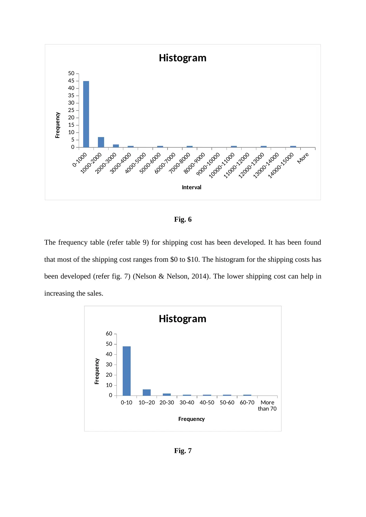
The frequency table (refer table 8) for sales is developed. It has been found that most of the
sales ranges from $0 to $1000. The histogram for the sales has been developed (refer fig. 6).

0-1000
1000-2000
2000-3000
3000-4000
4000-5000
5000-6000
6000-7000
7000-8000
8000-9000
9000-10000
10000-11000
11000-12000
12000-13000
13000-14000
14000-15000
More
0
5
10
15
20
25
30
35
40
45
50
Histogram
Interval
Frequency
Fig. 6
The frequency table (refer table 9) for shipping cost has been developed. It has been found
that most of the shipping cost ranges from $0 to $10. The histogram for the shipping costs has
been developed (refer fig. 7) (Nelson & Nelson, 2014). The lower shipping cost can help in
increasing the sales.
0-10 10--20 20-30 30-40 40-50 50-60 60-70 More
than 70
0
10
20
30
40
50
60
Histogram
Frequency
Frequency
Fig. 7

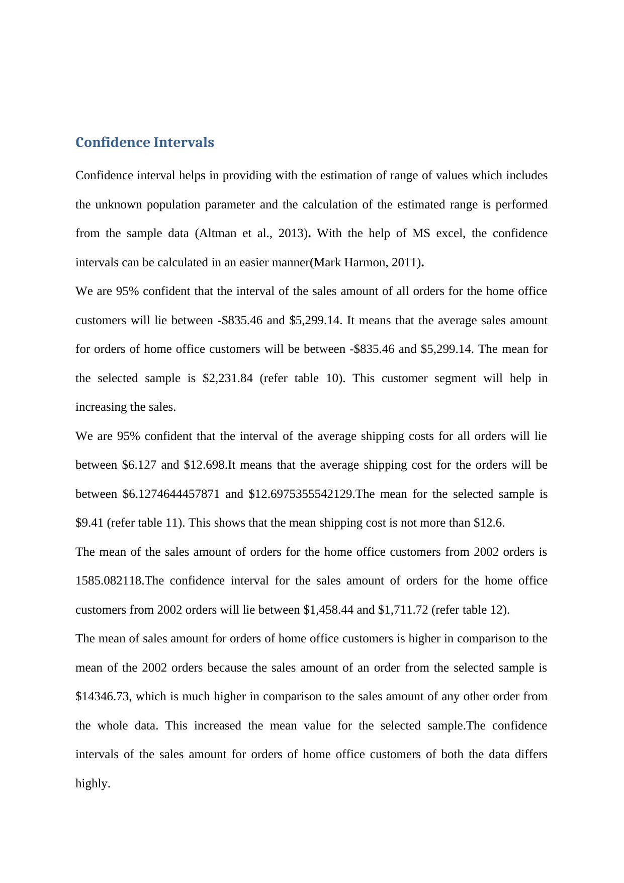
Confidence Intervals
Confidence interval helps in providing with the estimation of range of values which includes
the unknown population parameter and the calculation of the estimated range is performed
from the sample data (Altman et al., 2013). With the help of MS excel, the confidence
intervals can be calculated in an easier manner(Mark Harmon, 2011).
We are 95% confident that the interval of the sales amount of all orders for the home office
customers will lie between -$835.46 and $5,299.14. It means that the average sales amount
for orders of home office customers will be between -$835.46 and $5,299.14. The mean for
the selected sample is $2,231.84 (refer table 10). This customer segment will help in
increasing the sales.
We are 95% confident that the interval of the average shipping costs for all orders will lie
between $6.127 and $12.698.It means that the average shipping cost for the orders will be
between $6.1274644457871 and $12.6975355542129.The mean for the selected sample is
$9.41 (refer table 11). This shows that the mean shipping cost is not more than $12.6.
The mean of the sales amount of orders for the home office customers from 2002 orders is
1585.082118.The confidence interval for the sales amount of orders for the home office
customers from 2002 orders will lie between $1,458.44 and $1,711.72 (refer table 12).
The mean of sales amount for orders of home office customers is higher in comparison to the
mean of the 2002 orders because the sales amount of an order from the selected sample is
$14346.73, which is much higher in comparison to the sales amount of any other order from
the whole data. This increased the mean value for the selected sample.The confidence
intervals of the sales amount for orders of home office customers of both the data differs
highly.

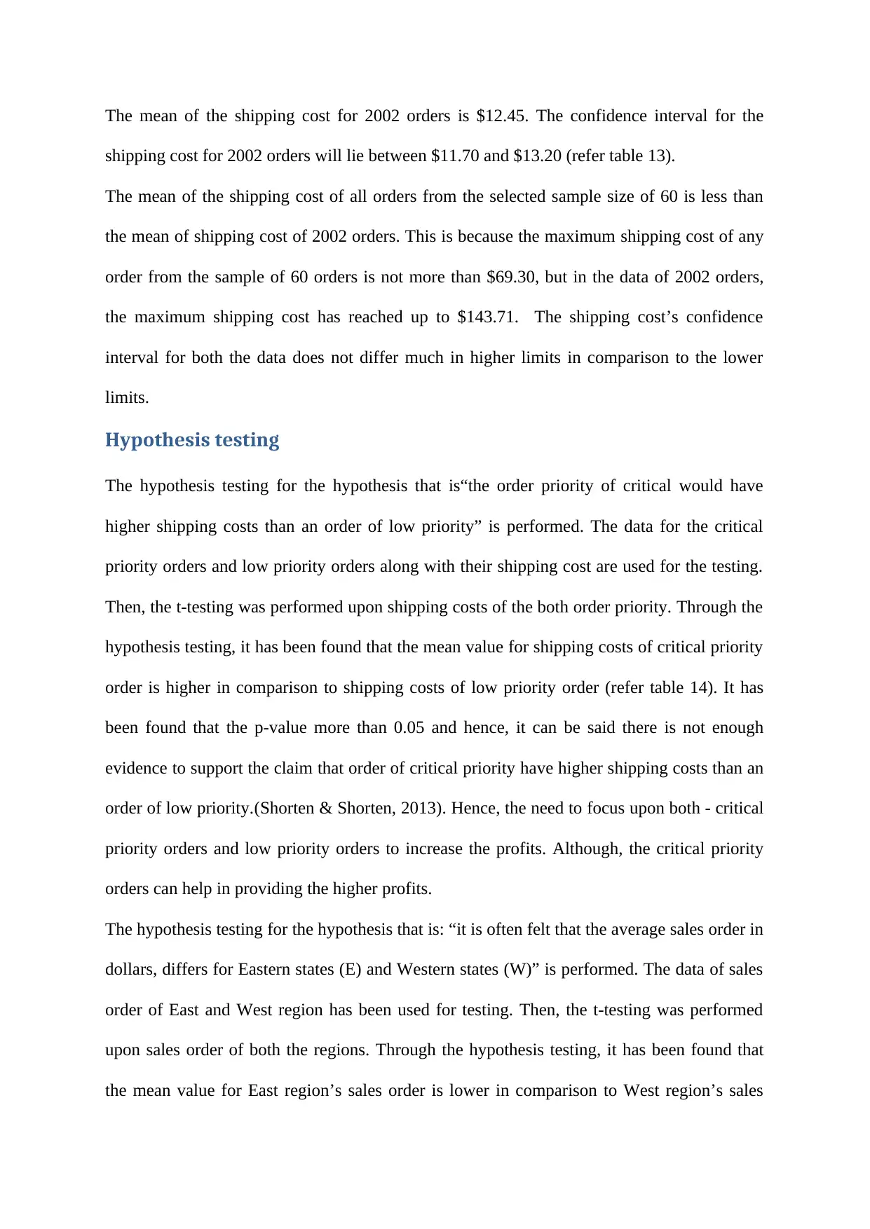
The mean of the shipping cost for 2002 orders is $12.45. The confidence interval for the
shipping cost for 2002 orders will lie between $11.70 and $13.20 (refer table 13).
The mean of the shipping cost of all orders from the selected sample size of 60 is less than
the mean of shipping cost of 2002 orders. This is because the maximum shipping cost of any
order from the sample of 60 orders is not more than $69.30, but in the data of 2002 orders,
the maximum shipping cost has reached up to $143.71. The shipping cost’s confidence
interval for both the data does not differ much in higher limits in comparison to the lower
limits.
Hypothesis testing
The hypothesis testing for the hypothesis that is“the order priority of critical would have
higher shipping costs than an order of low priority” is performed. The data for the critical
priority orders and low priority orders along with their shipping cost are used for the testing.
Then, the t-testing was performed upon shipping costs of the both order priority. Through the
hypothesis testing, it has been found that the mean value for shipping costs of critical priority
order is higher in comparison to shipping costs of low priority order (refer table 14). It has
been found that the p-value more than 0.05 and hence, it can be said there is not enough
evidence to support the claim that order of critical priority have higher shipping costs than an
order of low priority.(Shorten & Shorten, 2013). Hence, the need to focus upon both - critical
priority orders and low priority orders to increase the profits. Although, the critical priority
orders can help in providing the higher profits.
The hypothesis testing for the hypothesis that is: “it is often felt that the average sales order in
dollars, differs for Eastern states (E) and Western states (W)” is performed. The data of sales
order of East and West region has been used for testing. Then, the t-testing was performed
upon sales order of both the regions. Through the hypothesis testing, it has been found that
the mean value for East region’s sales order is lower in comparison to West region’s sales

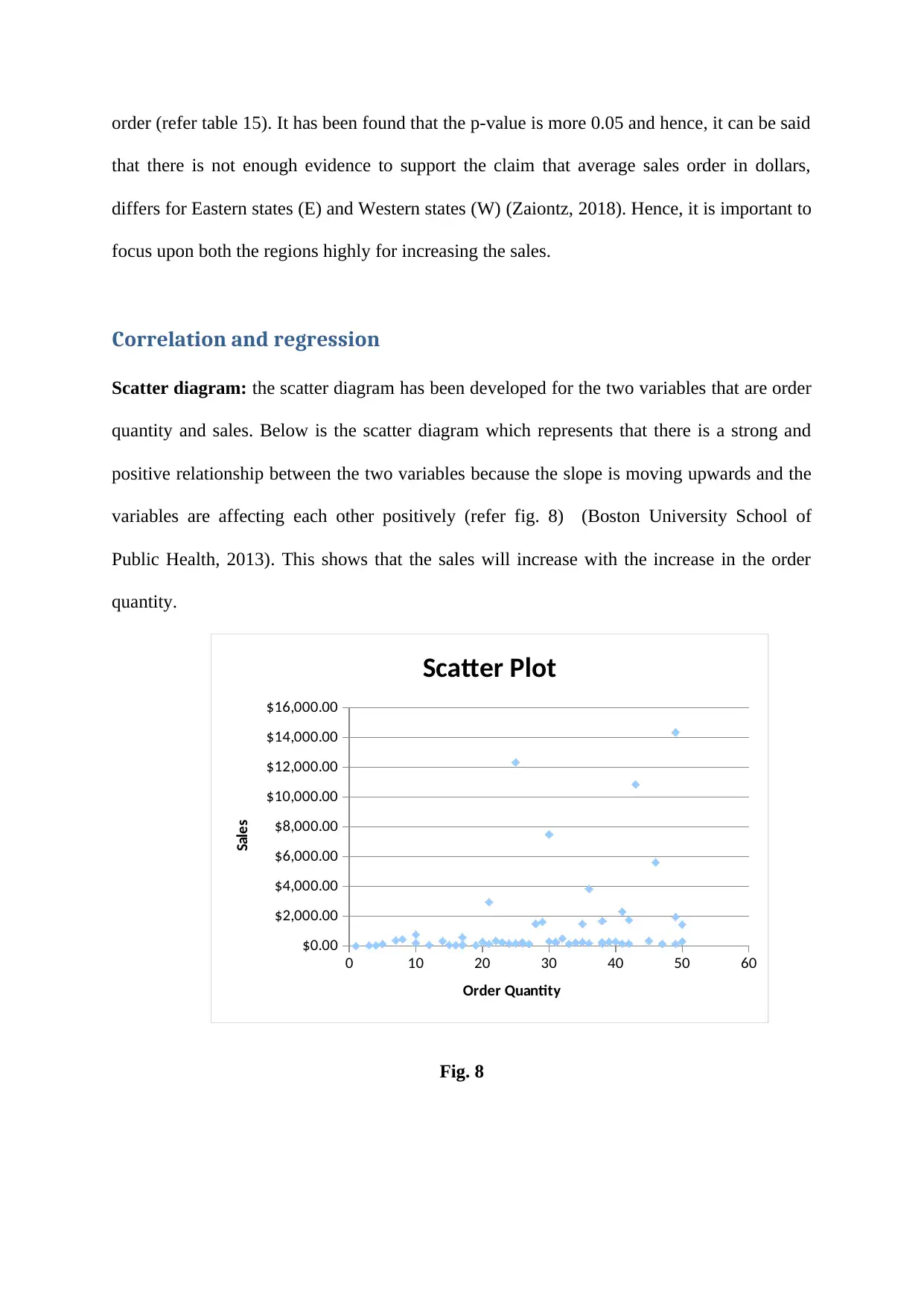
order (refer table 15). It has been found that the p-value is more 0.05 and hence, it can be said
that there is not enough evidence to support the claim that average sales order in dollars,
differs for Eastern states (E) and Western states (W) (Zaiontz, 2018). Hence, it is important to
focus upon both the regions highly for increasing the sales.
Correlation and regression
Scatter diagram: the scatter diagram has been developed for the two variables that are order
quantity and sales. Below is the scatter diagram which represents that there is a strong and
positive relationship between the two variables because the slope is moving upwards and the
variables are affecting each other positively (refer fig. 8) (Boston University School of
Public Health, 2013). This shows that the sales will increase with the increase in the order
quantity.
0 10 20 30 40 50 60
$0.00
$2,000.00
$4,000.00
$6,000.00
$8,000.00
$10,000.00
$12,000.00
$14,000.00
$16,000.00
Scatter Plot
Order Quantity
Sales
Fig. 8

For analyzing the relationship between the sales in dollars and order quantity, correlation and
regression has been performed. The multiple r value represents that there is a strong and
positive relationship between both the variables (refer table 16). This shows that the sales in
dollars will increase if the order quantity increases by multiple of 0.29.
Coefficients of correlation and determination
Coefficient of correlation shows that the variables are moving in unison and there is weak
positive linear correlation between the variables (Mathsbit, 2018). This shows that the
increase in one variable will also increase the other variable.
Coefficient of determination denotes that the strength of the linear association between the
variables (Sullivan, 2018). The r2 value shows that sales explain 8.7% variation in order
quantity. The R square value shows that the order quantity can bring the less variation in the
sales in comparison to the other variables of the data set.
Hypothesis testing
The hypothesis testing is performed in order to see whether or not that there is linear
relationship between sales and order quantity for an order. From the regression table, we can
see that p-value for coefficient of sales is less than 0.05. This shows that there significant
linear relationship between sales and order quantity. The increase in the order quantity can
help in increasing the sales in an effective manner.
Conclusion
The selected sample of the orders is arranged using the data summary methods. The data are
presented in the form of pie charts and the frequency tables in order to identify the total
number of occurrence of the specific criteria in the data. The confidence intervals of the sales