Economic Growth Analysis: Household Spending & Government Policies

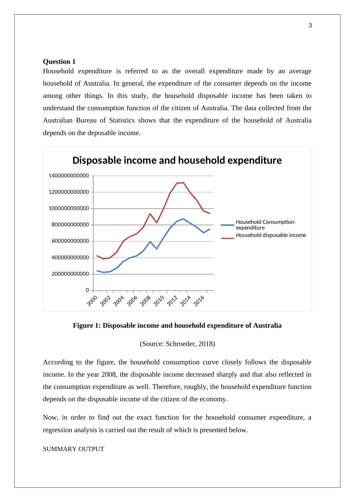
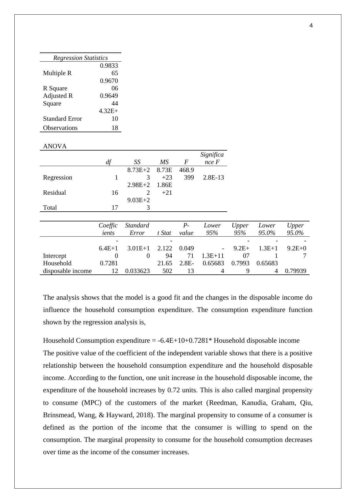
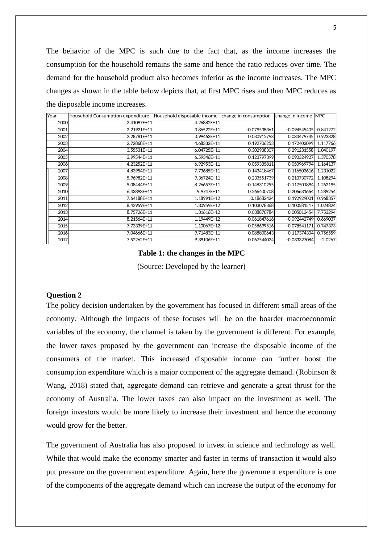
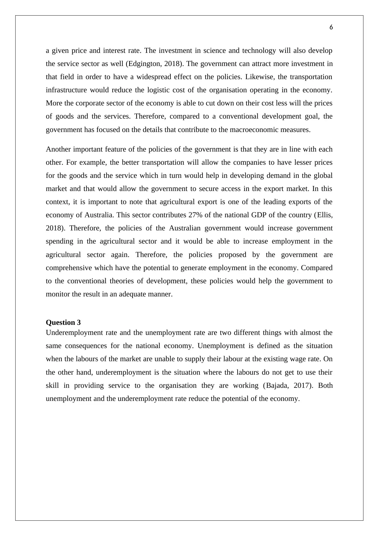
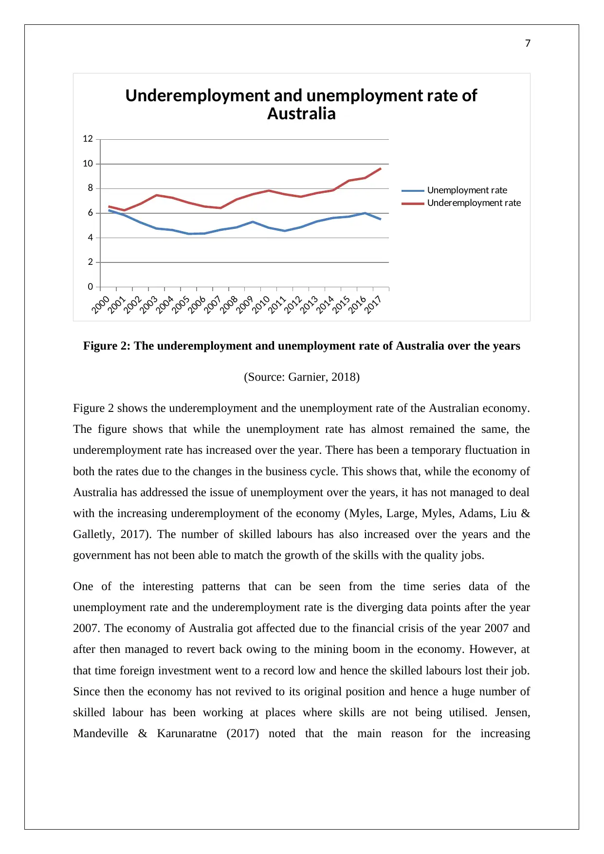
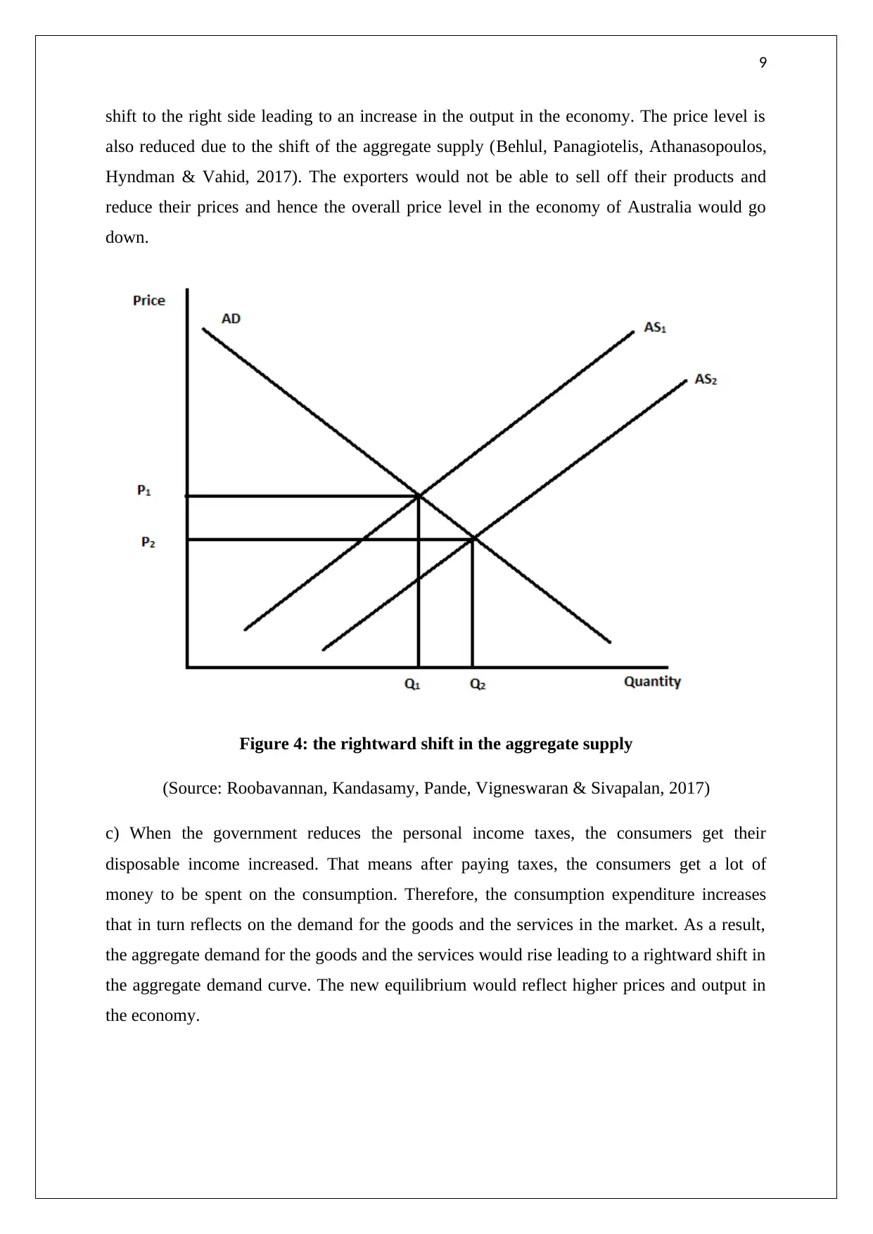
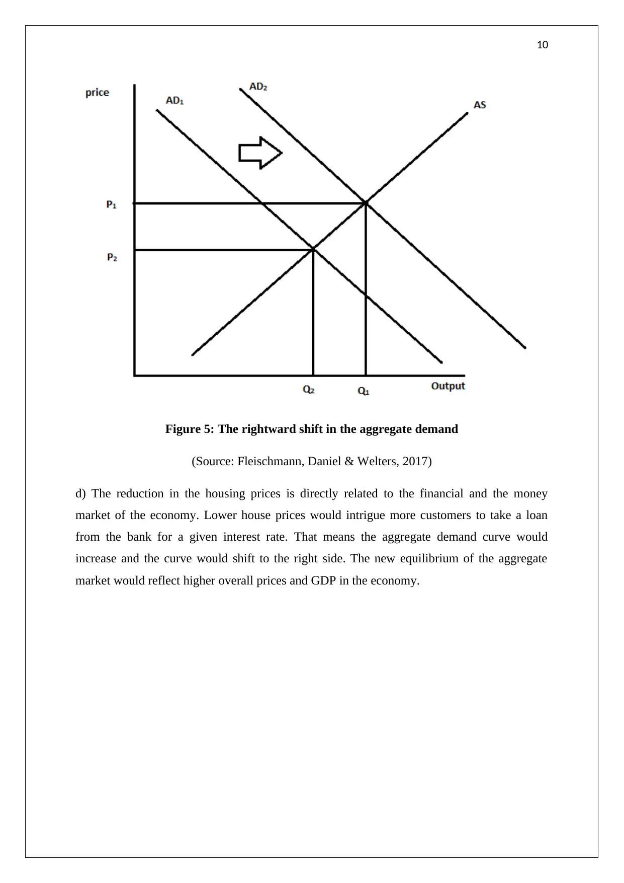
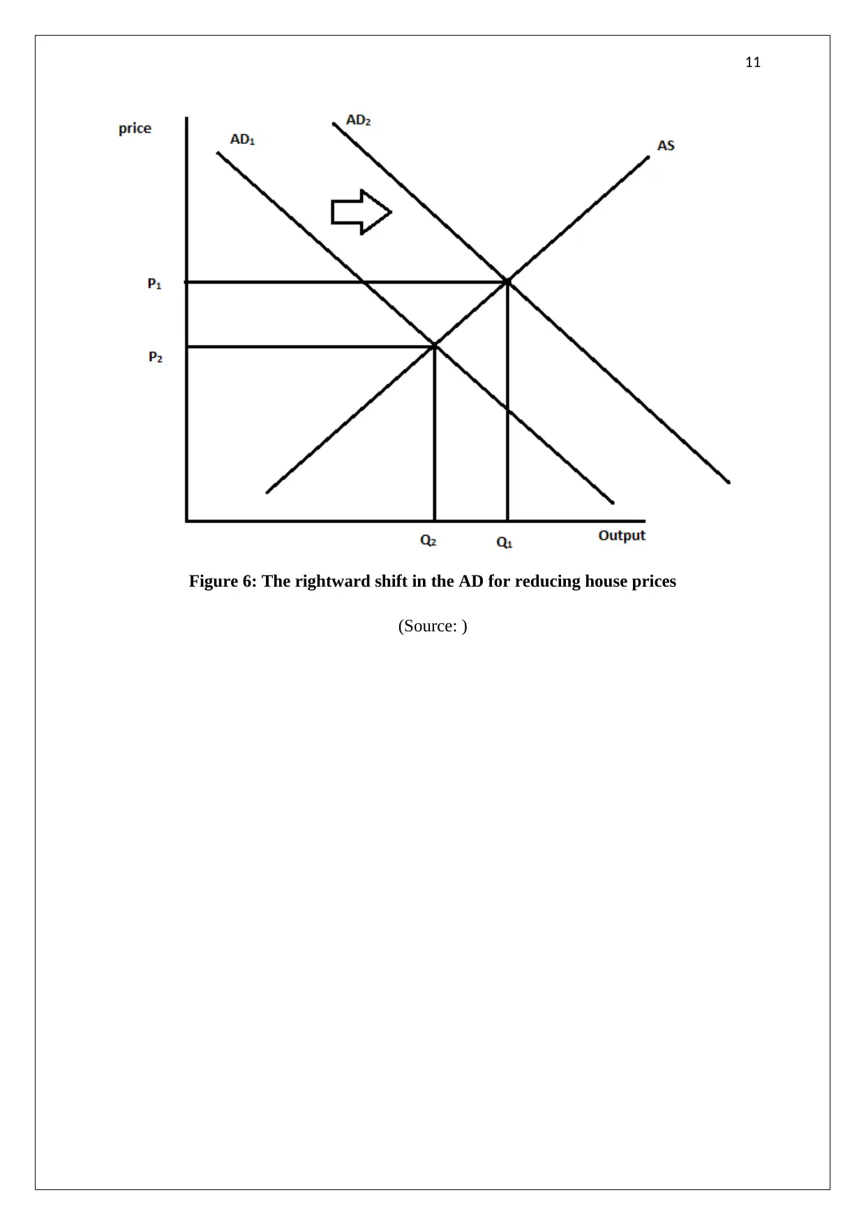
This assignment delves into the economic landscape of Australia, analyzing the intricate relationship between household expenditure, government policies, and overall economic growth. It begins by examining the household consumption function, utilizing data from the Australian Bureau of Statistics to model the connection between disposable income and consumption expenditure, further calculating and interpreting the marginal propensity to consume (MPC) over time. The assignment then evaluates the Australian government's strategies for promoting economic growth, particularly focusing on initiatives like lower taxes, investments in science and technology, infrastructure development, and agricultural support. It contrasts these policies with standard economic determinants of growth, highlighting the government's emphasis on detailed, interconnected approaches. Furthermore, the study investigates the issues of unemployment and underemployment in Australia, noting the divergence between these rates and the challenges in matching skilled labor with quality jobs. Finally, the assignment analyzes the potential impacts of various economic factors, such as changes in electricity prices, US trade policies, personal income taxes, and housing prices, on the aggregate supply and demand within the Australian economy, providing a comprehensive overview of the key drivers and challenges facing the nation's economic development.

1
ECONOMICS ASSIGNMENT

2
Contents
Question 1..................................................................................................................................3
Question 2..................................................................................................................................5
Question 3..................................................................................................................................6
Question 4..................................................................................................................................8
Reference..................................................................................................................................12

3
Question 1
Household expenditure is referred to as the overall expenditure made by an average
household of Australia. In general, the expenditure of the consumer depends on the income
among other things. In this study, the household disposable income has been taken to
understand the consumption function of the citizen of Australia. The data collected from the
Australian Bureau of Statistics shows that the expenditure of the household of Australia
depends on the deposable income.
2000
2002
2004
2006
2008
2010
2012
2014
2016
0
200000000000
400000000000
600000000000
800000000000
1000000000000
1200000000000
1400000000000
Disposable income and household expenditure
Household Consumption
expenditure
Household disposable income
Figure 1: Disposable income and household expenditure of Australia
(Source: Schroeder, 2018)
According to the figure, the household consumption curve closely follows the disposable
income. In the year 2008, the disposable income decreased sharply and that also reflected in
the consumption expenditure as well. Therefore, roughly, the household expenditure function
depends on the disposable income of the citizen of the economy.
Now, in order to find out the exact function for the household consumer expenditure, a
regression analysis is carried out the result of which is presented below.
SUMMARY OUTPUT

4
Regression Statistics
Multiple R
0.9833
65
R Square
0.9670
06
Adjusted R
Square
0.9649
44
Standard Error
4.32E+
10
Observations 18
ANOVA
df SS MS F
Significa
nce F
Regression 1
8.73E+2
3
8.73E
+23
468.9
399 2.8E-13
Residual 16
2.98E+2
2
1.86E
+21
Total 17
9.03E+2
3
Coeffic
ients
Standard
Error t Stat
P-
value
Lower
95%
Upper
95%
Lower
95.0%
Upper
95.0%
Intercept
-
6.4E+1
0
3.01E+1
0
-
2.122
94
0.049
71
-
1.3E+11
-
9.2E+
07
-
1.3E+1
1
-
9.2E+0
7
Household
disposable income
0.7281
12 0.033623
21.65
502
2.8E-
13
0.65683
4
0.7993
9
0.65683
4 0.79939
The analysis shows that the model is a good fit and the changes in the disposable income do
influence the household consumption expenditure. The consumption expenditure function
shown by the regression analysis is,
Household Consumption expenditure = -6.4E+10+0.7281* Household disposable income
The positive value of the coefficient of the independent variable shows that there is a positive
relationship between the household consumption expenditure and the household disposable
income. According to the function, one unit increase in the household disposable income, the
expenditure of the household increases by 0.72 units. This is also called marginal propensity
to consume (MPC) of the customers of the market (Reedman, Kanudia, Graham, Qiu,
Brinsmead, Wang, & Hayward, 2018). The marginal propensity to consume of a consumer is
defined as the portion of the income that the consumer is willing to spend on the
consumption. The marginal propensity to consume for the household consumption decreases
over time as the income of the consumer increases.

5
The behavior of the MPC is such due to the fact that, as the income increases the
consumption for the household remains the same and hence the ratio reduces over time. The
demand for the household product also becomes inferior as the income increases. The MPC
changes as shown in the table below depicts that, at first MPC rises and then MPC reduces as
the disposable income increases.
Year Household Consumption expenditure Household disposable income change in consumption change in income MPC
2000 2.41097E+11 4.26882E+11
2001 2.21921E+11 3.86522E+11 -0.079538361 -0.094545405 0.841272
2002 2.28781E+11 3.99463E+11 0.030912793 0.033479745 0.923328
2003 2.72868E+11 4.68332E+11 0.192706253 0.172403099 1.117766
2004 3.55531E+11 6.04725E+11 0.302938307 0.291231558 1.040197
2005 3.99544E+11 6.59346E+11 0.123797399 0.090324927 1.370578
2006 4.23252E+11 6.92953E+11 0.059335811 0.050969794 1.164137
2007 4.83954E+11 7.73685E+11 0.143418467 0.116503616 1.231022
2008 5.96982E+11 9.36724E+11 0.233551739 0.210730772 1.108294
2009 5.08444E+11 8.26657E+11 -0.148310255 -0.117501894 1.262195
2010 6.43893E+11 9.9747E+11 0.266400708 0.206631664 1.289254
2011 7.64188E+11 1.18991E+12 0.18682424 0.192929001 0.968357
2012 8.42959E+11 1.30959E+12 0.103078368 0.100581517 1.024824
2013 8.75726E+11 1.31616E+12 0.038870784 0.005013454 7.753294
2014 8.21564E+11 1.19449E+12 -0.061847616 -0.092442749 0.669037
2015 7.73339E+11 1.10067E+12 -0.058699516 -0.078541171 0.747373
2016 7.04666E+11 9.71483E+11 -0.088800643 -0.117374304 0.756559
2017 7.52262E+11 9.39106E+11 0.067544024 -0.033327084 -2.0267
Table 1: the changes in the MPC
(Source: Developed by the learner)
Question 2
The policy decision undertaken by the government has focused in different small areas of the
economy. Although the impacts of these focuses will be on the boarder macroeconomic
variables of the economy, the channel is taken by the government is different. For example,
the lower taxes proposed by the government can increase the disposable income of the
consumers of the market. This increased disposable income can further boost the
consumption expenditure which is a major component of the aggregate demand. (Robinson &
Wang, 2018) stated that, aggregate demand can retrieve and generate a great thrust for the
economy of Australia. The lower taxes can also impact on the investment as well. The
foreign investors would be more likely to increase their investment and hence the economy
would grow for the better.
The government of Australia has also proposed to invest in science and technology as well.
While that would make the economy smarter and faster in terms of transaction it would also
put pressure on the government expenditure. Again, here the government expenditure is one
of the components of the aggregate demand which can increase the output of the economy for

6
a given price and interest rate. The investment in science and technology will also develop
the service sector as well (Edgington, 2018). The government can attract more investment in
that field in order to have a widespread effect on the policies. Likewise, the transportation
infrastructure would reduce the logistic cost of the organisation operating in the economy.
More the corporate sector of the economy is able to cut down on their cost less will the prices
of goods and the services. Therefore, compared to a conventional development goal, the
government has focused on the details that contribute to the macroeconomic measures.
Another important feature of the policies of the government is that they are in line with each
other. For example, the better transportation will allow the companies to have lesser prices
for the goods and the service which in turn would help in developing demand in the global
market and that would allow the government to secure access in the export market. In this
context, it is important to note that agricultural export is one of the leading exports of the
economy of Australia. This sector contributes 27% of the national GDP of the country (Ellis,
2018). Therefore, the policies of the Australian government would increase government
spending in the agricultural sector and it would be able to increase employment in the
agricultural sector again. Therefore, the policies proposed by the government are
comprehensive which have the potential to generate employment in the economy. Compared
to the conventional theories of development, these policies would help the government to
monitor the result in an adequate manner.
Question 3
Underemployment rate and the unemployment rate are two different things with almost the
same consequences for the national economy. Unemployment is defined as the situation
when the labours of the market are unable to supply their labour at the existing wage rate. On
the other hand, underemployment is the situation where the labours do not get to use their
skill in providing service to the organisation they are working (Bajada, 2017). Both
unemployment and the underemployment rate reduce the potential of the economy.

7
2000
2001
2002
2003
2004
2005
2006
2007
2008
2009
2010
2011
2012
2013
2014
2015
2016
2017
0
2
4
6
8
10
12
Underemployment and unemployment rate of
Australia
Unemployment rate
Underemployment rate
Figure 2: The underemployment and unemployment rate of Australia over the years
(Source: Garnier, 2018)
Figure 2 shows the underemployment and the unemployment rate of the Australian economy.
The figure shows that while the unemployment rate has almost remained the same, the
underemployment rate has increased over the year. There has been a temporary fluctuation in
both the rates due to the changes in the business cycle. This shows that, while the economy of
Australia has addressed the issue of unemployment over the years, it has not managed to deal
with the increasing underemployment of the economy (Myles, Large, Myles, Adams, Liu &
Galletly, 2017). The number of skilled labours has also increased over the years and the
government has not been able to match the growth of the skills with the quality jobs.
One of the interesting patterns that can be seen from the time series data of the
unemployment rate and the underemployment rate is the diverging data points after the year
2007. The economy of Australia got affected due to the financial crisis of the year 2007 and
after then managed to revert back owing to the mining boom in the economy. However, at
that time foreign investment went to a record low and hence the skilled labours lost their job.
Since then the economy has not revived to its original position and hence a huge number of
skilled labour has been working at places where skills are not being utilised. Jensen,
Mandeville & Karunaratne (2017) noted that the main reason for the increasing

8
underemployment in Australia is the low aggregate demand following the global financial
crisis and the end of the mining boom.
Question 4
a) Electricity is used in almost all the major businesses of the economy. The supply side of
the economy used electricity as one of the inputs to the production process. Therefore the
increase in the price of electricity would increase the cost of operation of the businesses in the
market (Robinson, Atkin, Caputo & Wang, 2017). Consequently, the number of goods or
services sold at a given price would reduce leading to a leftward shift in the aggregate
demand. The new equilibrium of the market will reflect a higher price for the goods and the
services and the lower output in the economy.
Figure 3: The leftward shift in the aggregate supply
(Source: Hudson & Wood, 2017)
b) If the USA government imposes taxes for the export of Australia to the market of USA, the
products and services intended to be sold in the market of USA would not be sold and hence
the aggregate supply in Australia would rise. This would shift the aggregate supply curve to

9
shift to the right side leading to an increase in the output in the economy. The price level is
also reduced due to the shift of the aggregate supply (Behlul, Panagiotelis, Athanasopoulos,
Hyndman & Vahid, 2017). The exporters would not be able to sell off their products and
reduce their prices and hence the overall price level in the economy of Australia would go
down.
Figure 4: the rightward shift in the aggregate supply
(Source: Roobavannan, Kandasamy, Pande, Vigneswaran & Sivapalan, 2017)
c) When the government reduces the personal income taxes, the consumers get their
disposable income increased. That means after paying taxes, the consumers get a lot of
money to be spent on the consumption. Therefore, the consumption expenditure increases
that in turn reflects on the demand for the goods and the services in the market. As a result,
the aggregate demand for the goods and the services would rise leading to a rightward shift in
the aggregate demand curve. The new equilibrium would reflect higher prices and output in
the economy.

10
Figure 5: The rightward shift in the aggregate demand
(Source: Fleischmann, Daniel & Welters, 2017)
d) The reduction in the housing prices is directly related to the financial and the money
market of the economy. Lower house prices would intrigue more customers to take a loan
from the bank for a given interest rate. That means the aggregate demand curve would
increase and the curve would shift to the right side. The new equilibrium of the aggregate
market would reflect higher overall prices and GDP in the economy.

11
Figure 6: The rightward shift in the AD for reducing house prices
(Source: )

12
Reference
Bajada, C. (2017). Australia's Cash Economy: A Troubling Issue for Policymakers: A
Troubling Issue for Policymakers. Routledge.
Behlul, T., Panagiotelis, A., Athanasopoulos, G., Hyndman, R. J., & Vahid, F. (2017). The
Australian Macro Database: An online resource for macroeconomic research in
Australia. A journal of applied economics and policy, 72(1), 41-161.
Edgington, D. W. (2018). Japanese business down under Patterns of Japanese investment in
Australia. Routledge.
Ellis, L. (2018). Where is the growth going to come from?. Economic Papers: A journal of
applied economics and policy, 37(1), 4-16.
Fleischmann, K., Daniel, R., & Welters, R. (2017). Developing a regional economy through
creative industries: innovation capacity in a regional Australian city. Creative
Industries Journal, 10(2), 119-138.
Garnier, G. (2018). Creating industries of tomorrow through research and innovation. Appita
Journal: Journal of the Technical Association of the Australian and New Zealand
Pulp and Paper Industry, 71(2), 100.
Hudson, D., & Wood, P. (2017). Agtech and food tech: An expanding investment
sector. Australasian Biotechnology, 27(2), 36.
Jensen, R. C., Mandeville, T. D., & Karunaratne, N. D. (2017). Regional economic planning:
Generation of regional input-output analysis. Routledge.
Myles, N., Large, M., Myles, H., Adams, R., Liu, D., & Galletly, C. (2017). Australia's
economic transition, unemployment, suicide, and mental health needs. Australian &
New Zealand Journal of Psychiatry, 51(2), 119-123.
Reedman, L. J., Kanudia, A., Graham, P. W., Qiu, J., Brinsmead, T. S., Wang, D., &
Hayward, J. A. (2018). Towards Zero Carbon Scenarios for the Australian Economy.
In Limiting Global Warming to Well Below 2° C: Energy System Modelling and
Policy Development (pp. 261-276). Springer, Cham.