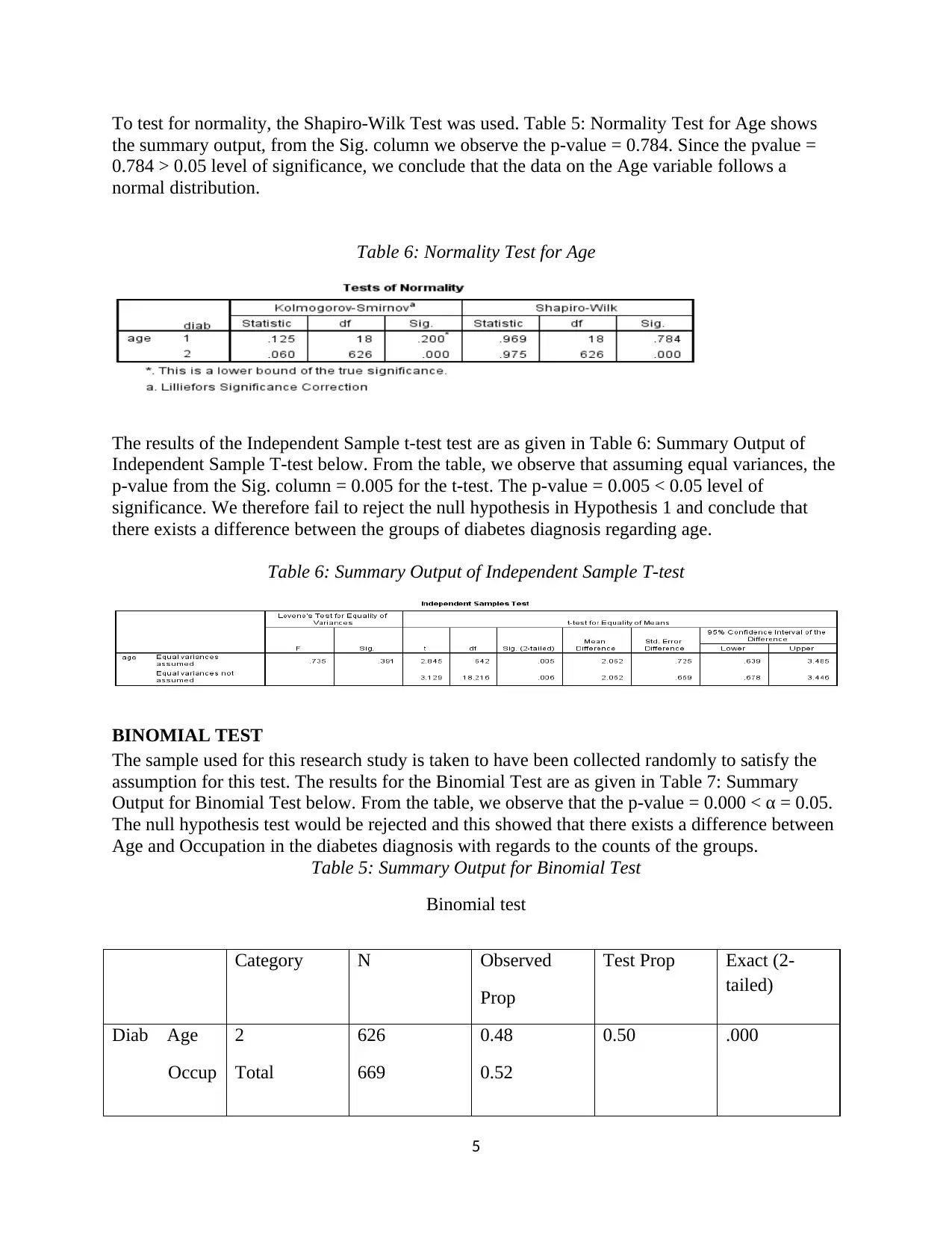
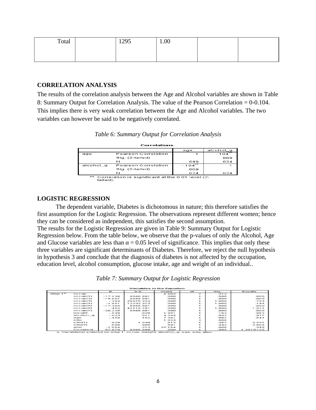
Analysis of Factors Influencing Diabetes Diagnosis: Research Report

This report presents a research study investigating the factors influencing the diagnosis of diabetes. The study aimed to determine the impact of occupation, education level, alcohol consumption, glucose intake, age, and weight on diabetes diagnosis. The research utilized several statistical methods, in...Read More

INTRODUCTION
RESEARCH QUESTIONS
The research question for this study is: Is the diagnosis of diabetes affected by the occupation,
education level, alcohol consumption, glucose intake, age and weight of an individual?
RESEARCH OBJECTIVES
The main objective of this research study is:
To determine whether the diagnosis of diabetes is affected by the occupation, education level,
alcohol consumption, glucose intake, age and weight of an individual.
The other objectives in this study are:
1. To determine whether there is a difference between the categories of diabetes diagnosis
regarding age.
2. To determine whether the categories of diabetes diagnosis significantly differ from each other
based on counts.
.
RESEARCH HYPOTHESES
This research study will test three hypotheses:
HYPOTHESIS 1
Null Hypothesis (H0): The diagnosis of diabetes categories would significant differs from each
other based on age.
Alternative Hypothesis (H1): There isn’t any difference between the categories of diabetes
diagnosis regarding age.
In order to test this hypothesis, the Independent Sample t-test is applied. The t-test is a statistical
test that specifically provides information on the relationship between two variables with the
dependent being metric (measured on interval or ratio scale) and the independent being non
metric with two categories (measured on either nominal or ordinal scale) (Barbara & Susan,
2014; Ren & Ying, 2010).
The assumptions of the Independent Sample t-test are (Witten, 2011; Everitt &
Skrondal,2010):
1. The dependent variable should be continuous in nature. This implies that it should be
measured on either interval or ratio scales.
2. The independent variable should be categorical in nature with two or more groups.
3. The observations should be independent of each other.
4. The data should not contain outliers that can be considered as significant.
5. The dependent variable should follow a normal distribution.
1

HYPOTHESIS 2
Null Hypothesis (H0): The categories of diabetes diagnosis significantly differ from each other.
Alternative Hypothesis (H1): The categories of diabetes diagnosis do not significantly differ
from each other.
In order to test this hypothesis, the Binomial test is applied. The Binomial test is a form of a
probabilistic statistical test for testing difference between the categories of a dichotomous
variable (Usama & Padhraic, 2008). The Binomial test is a non-parametric statistical test and
therefore the assumptions that apply for the parametric tests do not apply for this test (Corder &
Foreman, 2009). The only assumption for the Binomial test is that the sample used is a random
sample (Oscar, 2009).
HYPOTHESIS 3
Null Hypothesis (H0): The diagnosis of diabetes is affected by the occupation, education level,
alcohol consumption, glucose intake, age and weight of an individual.
Alternative Hypothesis (H1): The diagnosis of diabetes is not affected by the occupation,
education level, alcohol consumption, glucose intake, age and weight of an individual.
In order to test this hypothesis, the Logistic Regression is applied. Regression analysis can
broadly be defined as a statistical analysis method whose aim is to establish the presence,
absence and type of relationship between variables (Galit, Peter, Inbal, Patel, & Kenneth, 2018;
Han & Jaiwei, 2011). The Logistic Regression is a type of regression analysis in which the
dependent variable is categorical in nature (Hosmer, 2013). The dependent variable(s) can be
either continuous or categorical. For this study, the Binomial Logistic Regression will be
specifically used.
RESULTS
DESCRIPTIVE STATISTICS
From Table 1: Descriptive Statistics for Continuous Variables we observe the summary statistics
for the continuous data variables in the study.
Table 1: Descriptive Statistics for Continuous Variables
The histograms for the continuous variables are as shown in the plots in Figure 1: Histogram for
Weight Variable to Figure 4: Histogram for Age below. In all the plots, the distributions appear
to be skewed to the left except for the age variable which displays a bell shaped density curve
and it’s hence normally distributed from visual inspection.
2

Figure 1: Histogram for Weight Variable Figure 2: Histogram for Glucose Variable
Figure 3: Histogram for Alcohol Variable Figure 4: Histogram for Age
Table 2: Overall Descriptive Statistics for Categorical Variables shows the count of the valid and
missing observations in the data for the categorical variables in the study.
The diabetes variable, education and occupation had both valid and missing values, the table 2
shows the number of count that were observed and the number of count that were missing on all
the three variable categories.
Table 2: Overall Descriptive Statistics for Categorical Variables
3

Table 3: Descriptive Statistics for Diabetes Variable shows summary descriptive statistics for the
diabetes variable with category 1 representing an affirmative diagnosis for diabetes (Yes) while
category 2 represents no diabetes diagnosis.
Table 3: Descriptive Statistics for Diabetes Variable
Table 4: Descriptive Statistics for Education Variable shows the summary descriptive statistics
for the education variable with category 1 representing elementary school, 2 representing high
school and 3 representing university (highest level of education attained).
Table 4: Descriptive Statistics for Education Variable
INFERENTIAL STATISTICS
INDEPENDENT SAMPLE T-TEST
To test the assumptions for this test, we first observe the variables; Diabetes (Independent
Variable) and Age (Dependent Variable). The dependent variable, Age, is continuous in nature
hence satisfying the first assumption. The independent variable, Diabetes, is categorical in nature
with 2 groups hence satisfying the second assumption. For the third assumption, the observations
represent different women, hence they can be considered as independent.
To check for outliers, the boxplot below in Figure 5: Boxplot for Diabetes and Age was used.
From the boxplot we observe that there are no outlier data points.
Figure 5: Boxplot for diabetes and age
4

To test for normality, the Shapiro-Wilk Test was used. Table 5: Normality Test for Age shows
the summary output, from the Sig. column we observe the p-value = 0.784. Since the pvalue =
0.784 > 0.05 level of significance, we conclude that the data on the Age variable follows a
normal distribution.
Table 6: Normality Test for Age
The results of the Independent Sample t-test test are as given in Table 6: Summary Output of
Independent Sample T-test below. From the table, we observe that assuming equal variances, the
p-value from the Sig. column = 0.005 for the t-test. The p-value = 0.005 < 0.05 level of
significance. We therefore fail to reject the null hypothesis in Hypothesis 1 and conclude that
there exists a difference between the groups of diabetes diagnosis regarding age.
Table 6: Summary Output of Independent Sample T-test
BINOMIAL TEST
The sample used for this research study is taken to have been collected randomly to satisfy the
assumption for this test. The results for the Binomial Test are as given in Table 7: Summary
Output for Binomial Test below. From the table, we observe that the p-value = 0.000 < α = 0.05.
The null hypothesis test would be rejected and this showed that there exists a difference between
Age and Occupation in the diabetes diagnosis with regards to the counts of the groups.
Table 5: Summary Output for Binomial Test
Binomial test
Category N Observed
Prop
Test Prop Exact (2-
tailed)
Diab Age
Occup
2
Total
626
669
0.48
0.52
0.50 .000
5

Total 1295 1.00
CORRELATION ANALYSIS
The results of the correlation analysis between the Age and Alcohol variables are shown in Table
8: Summary Output for Correlation Analysis. The value of the Pearson Correlation = 0-0.104.
This implies there is very weak correlation between the Age and Alcohol variables. The two
variables can however be said to be negatively correlated.
Table 6: Summary Output for Correlation Analysis
LOGISTIC REGRESSION
The dependent variable, Diabetes is dichotomous in nature; this therefore satisfies the
first assumption for the Logistic Regression. The observations represent different women; hence
they can be considered as independent, this satisfies the second assumption.
The results for the Logistic Regression are given in Table 9: Summary Output for Logistic
Regression below. From the table below, we observe that the p-values of only the Alcohol, Age
and Glucose variables are less than α = 0.05 level of significance. This implies that only these
three variables are significant determinants of Diabetes. Therefore, we reject the null hypothesis
in hypothesis 3 and conclude that the diagnosis of diabetes is not affected by the occupation,
education level, alcohol consumption, glucose intake, age and weight of an individual..
Table 7: Summary Output for Logistic Regression
6

CONCLUSION
From the analysis results presented in this research study, we can conclude that there exists a
difference between the groups of diabetes diagnosis regarding age. This means that the age of an
individual is significant in determining the diabetes diagnosis of that individual. We also note
that there exists a difference among the groups in the diabetes diagnosis in general.
This implies that there is a difference between those that are diagnosed with diabetes and those
that are not diagnosed with diabetes.
We observe that there is very little relationship between Age and Alcohol consumption for the
age group represented in this study. The Alcohol, Age and Glucose however form the key
determinants of the Diabetes diagnosis.
REFERENCES
Barbara, I., & Susan, D. (2014). Introductory Statistics (1st ed.). New York: OpenStax CNX.
Corder, G. W., & Foreman, D. I. (2009). Non Parametric Statistics for Non Statisticians. pp. 99-
105 (1st ed.). Hoboken: John Wiley & Sons.
Everitt, B. S., & Skrondal, A. (2010). Cambridge Dictionary of Statistics (4th ed.). London:
Cambridge University Press.
Galit, S., Peter, B. C., Inbal, Y., Patel, N. R., & Kenneth, L. C. (2018). Data Mining for Business
Analytics (1st ed.). New Delhi: John Wiley & Sons, Inc.
Han, K., & Jaiwei, P. (2011). Data Mining: Concepts and Techniques (3rd ed.). London: Morgan
Kaufman.
Hosmer, D. (2013). Applied Logistic Regression (1 ed.). Hoboken, New Jersey: Wiley.
Jorge, A. A., Angela, A., & Edson, Z. M. (2013). Robust Linear Regression Models: Use of
Stable Distribution for the Response Data. Open Journal of Statistics, 3, 3-5.
Oscar, M. (2009). A data mining and knowledge discovery process model (1st ed.). Vienna: Julio
Ponce.
Ren, J., & Ying, S. (2010). Research and Improvement of Clustering Algorithms in Data Mining.
2010 2nd International Conference on Signal Processing Systems.
Tri, D., & Jugal, K. (2015). Select Machine Learning Algorithms Using Regression Models. 2015
IEEE Conference.
Usama, F., & Padhraic, S. (2008). From data mining to Knowledge Discovery in Databases (4th
ed.). New York: CRC Press.
Witten, I. H. (2011). Data Mining: Practical Machine Learning Tools (3rd ed.). Sydney :
Morgan Kaufmann.
7