Data Analysis Project: Income Data Analysis and Business Implications

This data analysis project investigates family income using a dataset containing information on working hours, wages, education, and other factors for both husbands and wives. The analysis begins with exploratory data analysis, including histograms and scatterplots to visualize the data distribution and relationships between variables. The project then employs multiple linear regression to model family income, assessing the significance of various predictors. The analysis reveals evidence of multicollinearity, prompting the use of principal component analysis (PCA) to extract independent components. Subsequently, multiple linear regression is performed using the extracted components, and the results are interpreted, highlighting the significant predictors of family income. The project concludes with a discussion of the business implications of the findings, emphasizing the importance of key income drivers in business strategies. The project aims to provide insights into the factors influencing family income and their practical relevance.

Running head: Data analysis 1
Data Analysis
Course title:
Student name:
Tutor’s name:

2.1 Exploratory data analysis
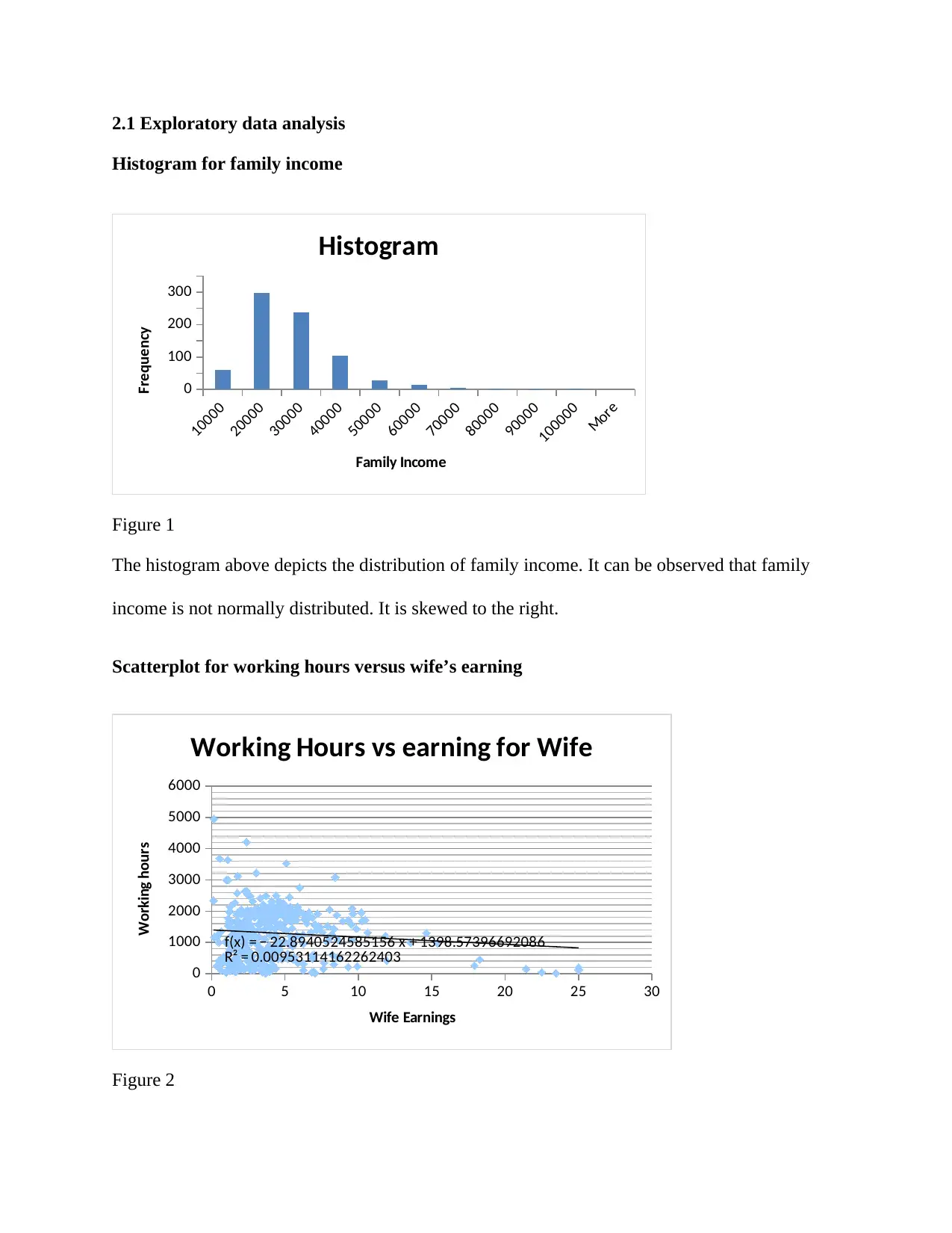
Histogram for family income
10000
20000
30000
40000
50000
60000
70000
80000
90000
100000
More
0
100
200
300
Histogram
Family Income
Frequency
Figure 1
The histogram above depicts the distribution of family income. It can be observed that family
income is not normally distributed. It is skewed to the right.
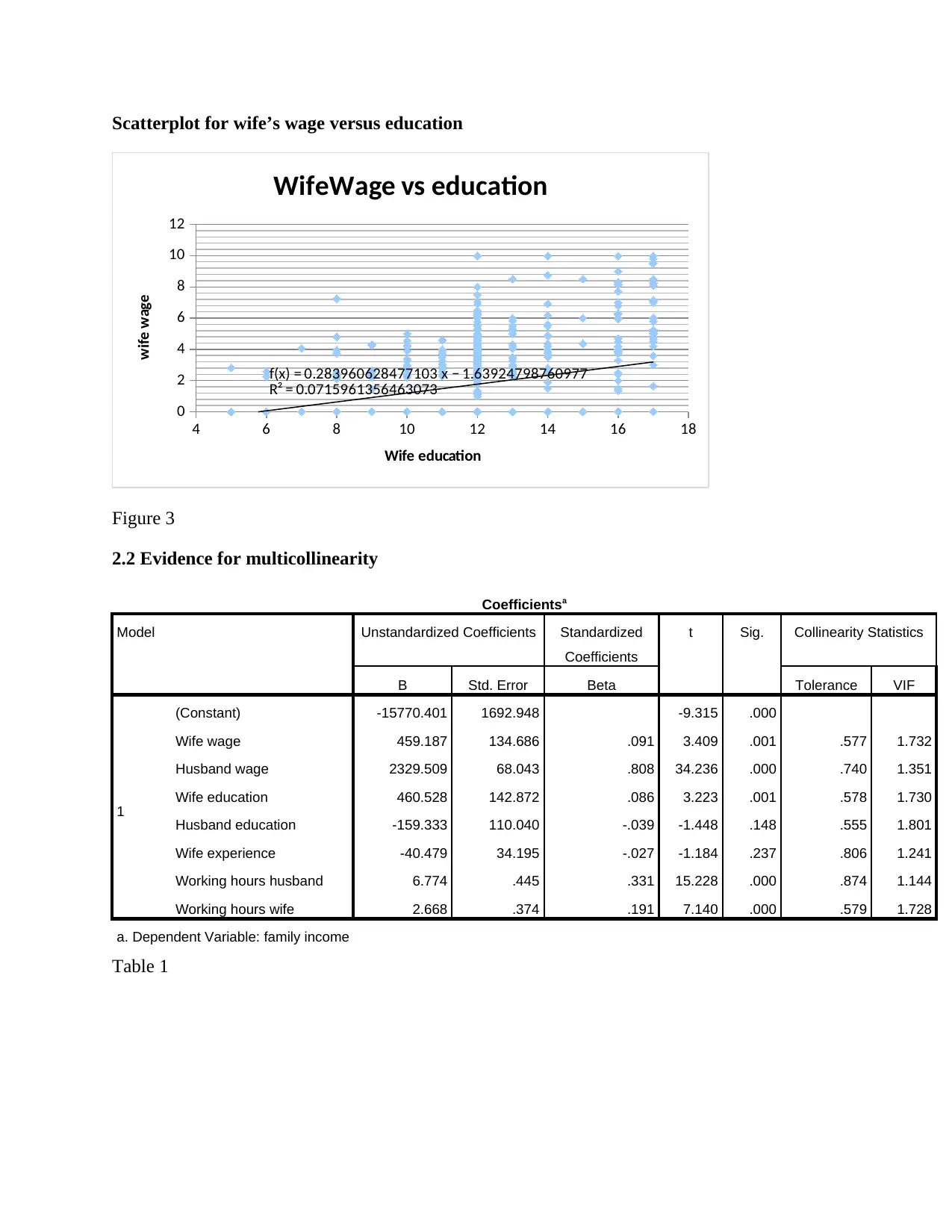
Scatterplot for working hours versus wife’s earning
0 5 10 15 20 25 30
0
1000
2000
3000
4000
5000
6000
f(x) = − 22.8940524585156 x + 1398.57396692086
R² = 0.00953114162262403
Working Hours vs earning for Wife
Wife Earnings
Working hours
Figure 2

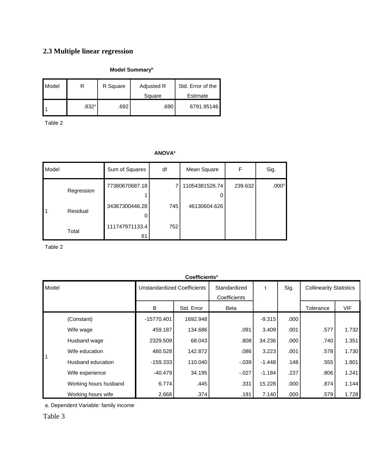
Scatterplot for wife’s wage versus education
4 6 8 10 12 14 16 18
0
2
4
6
8
10
12
f(x) = 0.283960628477103 x − 1.63924798760977
R² = 0.0715961356463073
WifeWage vs education
Wife education
wife wage
Figure 3
2.2 Evidence for multicollinearity
Coefficientsa
Model Unstandardized Coefficients Standardized
Coefficients
t Sig. Collinearity Statistics
B Std. Error Beta Tolerance VIF
1
(Constant) -15770.401 1692.948 -9.315 .000
Wife wage 459.187 134.686 .091 3.409 .001 .577 1.732
Husband wage 2329.509 68.043 .808 34.236 .000 .740 1.351
Wife education 460.528 142.872 .086 3.223 .001 .578 1.730
Husband education -159.333 110.040 -.039 -1.448 .148 .555 1.801
Wife experience -40.479 34.195 -.027 -1.184 .237 .806 1.241
Working hours husband 6.774 .445 .331 15.228 .000 .874 1.144
Working hours wife 2.668 .374 .191 7.140 .000 .579 1.728
a. Dependent Variable: family income
Table 1

2.3 Multiple linear regression
Model Summaryb
Model R R Square Adjusted R
Square
Std. Error of the
Estimate
1 .832a .692 .690 6791.95146
Table 2
ANOVAa
Model Sum of Squares df Mean Square F Sig.
1
Regression 77380670687.18
1
7 11054381526.74
0
239.632 .000b
Residual 34367300446.28
0
745 46130604.626
Total 111747971133.4
61
752
Table 2
Coefficientsa
Model Unstandardized Coefficients Standardized
Coefficients
t Sig. Collinearity Statistics
B Std. Error Beta Tolerance VIF
1
(Constant) -15770.401 1692.948 -9.315 .000
Wife wage 459.187 134.686 .091 3.409 .001 .577 1.732
Husband wage 2329.509 68.043 .808 34.236 .000 .740 1.351
Wife education 460.528 142.872 .086 3.223 .001 .578 1.730
Husband education -159.333 110.040 -.039 -1.448 .148 .555 1.801
Wife experience -40.479 34.195 -.027 -1.184 .237 .806 1.241
Working hours husband 6.774 .445 .331 15.228 .000 .874 1.144
Working hours wife 2.668 .374 .191 7.140 .000 .579 1.728
a. Dependent Variable: family income
Table 3

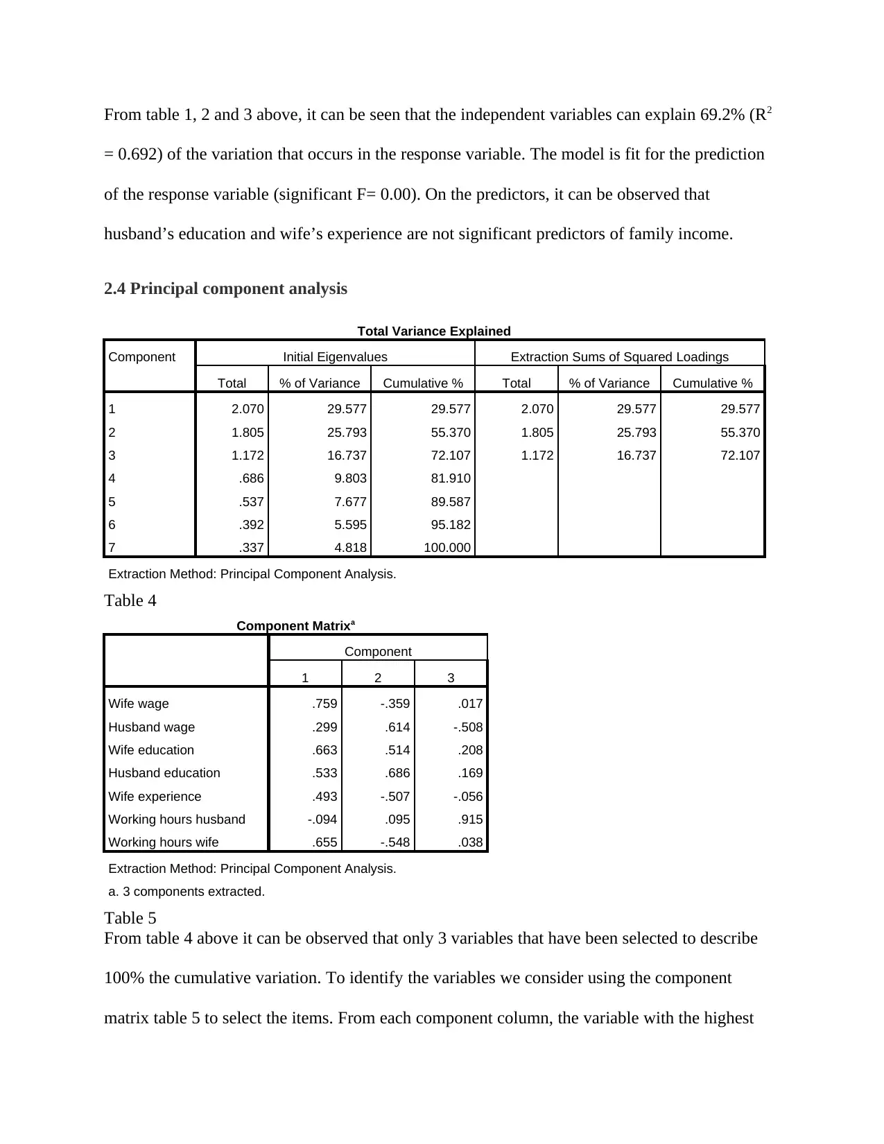
From table 1, 2 and 3 above, it can be seen that the independent variables can explain 69.2% (R2
= 0.692) of the variation that occurs in the response variable. The model is fit for the prediction
of the response variable (significant F= 0.00). On the predictors, it can be observed that
husband’s education and wife’s experience are not significant predictors of family income.
2.4 Principal component analysis
Total Variance Explained
Component Initial Eigenvalues Extraction Sums of Squared Loadings
Total % of Variance Cumulative % Total % of Variance Cumulative %
1 2.070 29.577 29.577 2.070 29.577 29.577
2 1.805 25.793 55.370 1.805 25.793 55.370
3 1.172 16.737 72.107 1.172 16.737 72.107
4 .686 9.803 81.910
5 .537 7.677 89.587
6 .392 5.595 95.182
7 .337 4.818 100.000
Extraction Method: Principal Component Analysis.
Table 4
Component Matrixa
Component
1 2 3
Wife wage .759 -.359 .017
Husband wage .299 .614 -.508
Wife education .663 .514 .208
Husband education .533 .686 .169
Wife experience .493 -.507 -.056
Working hours husband -.094 .095 .915
Working hours wife .655 -.548 .038
Extraction Method: Principal Component Analysis.
a. 3 components extracted.
Table 5
From table 4 above it can be observed that only 3 variables that have been selected to describe
100% the cumulative variation. To identify the variables we consider using the component
matrix table 5 to select the items. From each component column, the variable with the highest

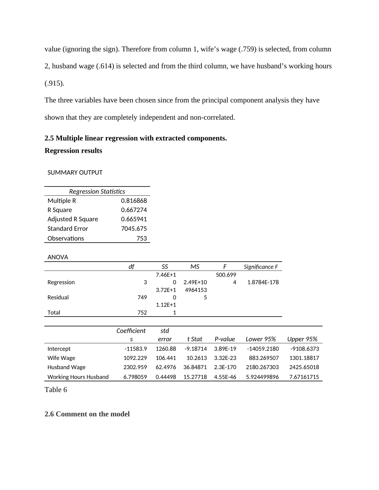
value (ignoring the sign). Therefore from column 1, wife’s wage (.759) is selected, from column
2, husband wage (.614) is selected and from the third column, we have husband’s working hours
(.915).
The three variables have been chosen since from the principal component analysis they have
shown that they are completely independent and non-correlated.
2.5 Multiple linear regression with extracted components.
Regression results
SUMMARY OUTPUT
Regression Statistics
Multiple R 0.816868
R Square 0.667274
Adjusted R Square 0.665941
Standard Error 7045.675
Observations 753
ANOVA
df SS MS F Significance F
Regression 3
7.46E+1
0 2.49E+10
500.699
4 1.8784E-178
Residual 749
3.72E+1
0
4964153
5
Total 752
1.12E+1
1
Coefficient
s
std
error t Stat P-value Lower 95% Upper 95%
Intercept -11583.9 1260.88 -9.18714 3.89E-19 -14059.2180 -9108.6373
Wife Wage 1092.229 106.441 10.2613 3.32E-23 883.269507 1301.18817
Husband Wage 2302.959 62.4976 36.84871 2.3E-170 2180.267303 2425.65018
Working Hours Husband 6.798059 0.44498 15.27718 4.55E-46 5.924499896 7.67161715
Table 6
2.6 Comment on the model

The table above shows the results of the regression analysis with the three extracted independent
variables (wife’s wage, husband’s wage and husband’s working hours). It can be observed that
the R2 value is 0.667. This means that the independent variables are responsible for 66.7% of the
variation that occurs in the response variable. It can also be observed that all independent
variables are significant predictors since all of them have p-values less than 0.05. To add on, a
unit change in wife’s wage causes a 1092.2 increase in family income. A unit change in
husband’s wage causes a 2302.96 increase in family income. Lastly, a unit change in husband’s
working hours causes a 6.8 increase in family income.
2.7 Business implication on the model
Contrary to business relying on factors such as wage per hour, numbers of hours worked by both
husband and wife, education and experience, the model reveals that the most significant
predictors are wife’s wage, husband’s wage and husband’s working hours. So if the most
important variables that are the drivers of the business are left out, then this may impact
negatively on the business.