University Assignment: Finite Element Method (Part 1) Solution

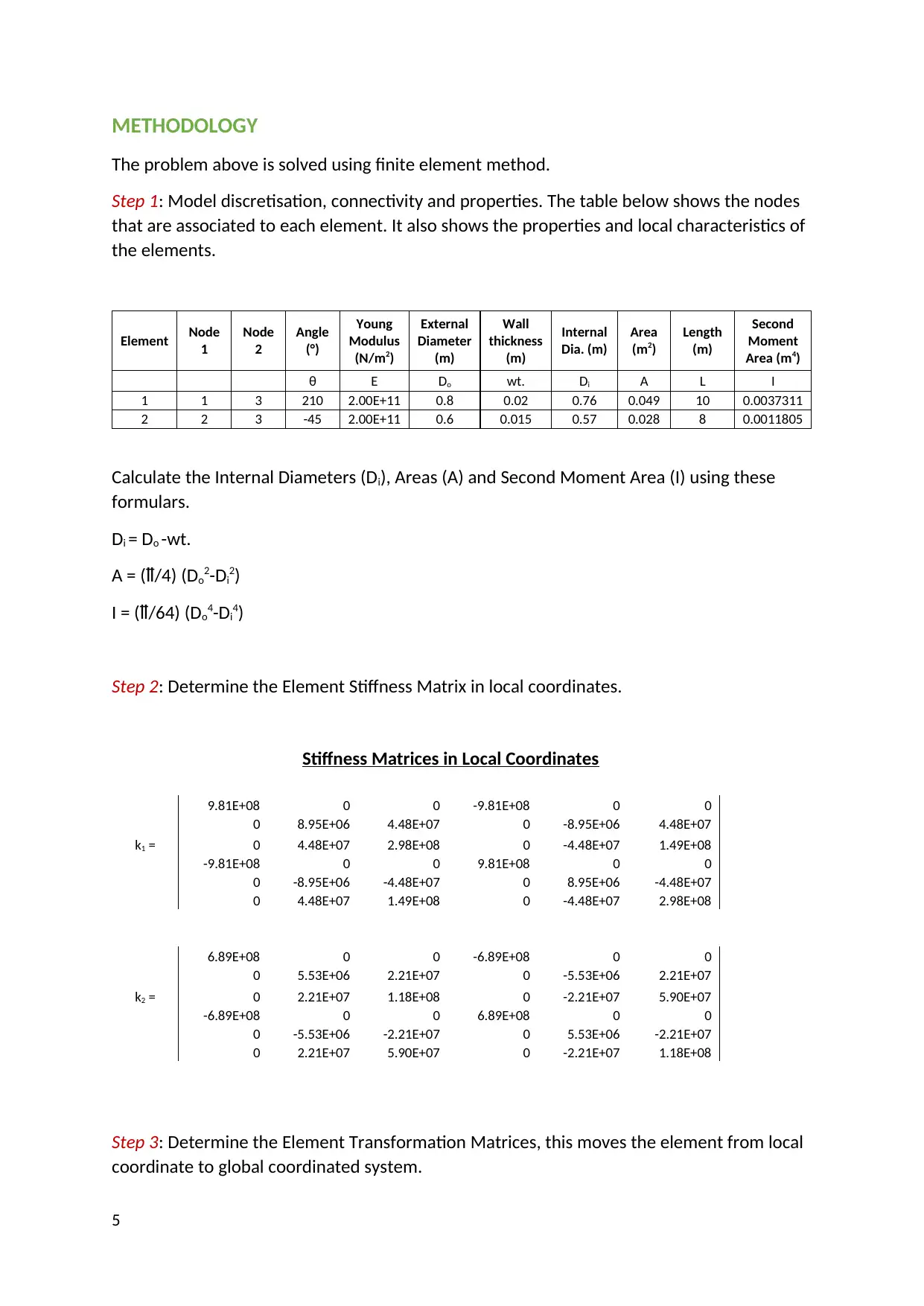
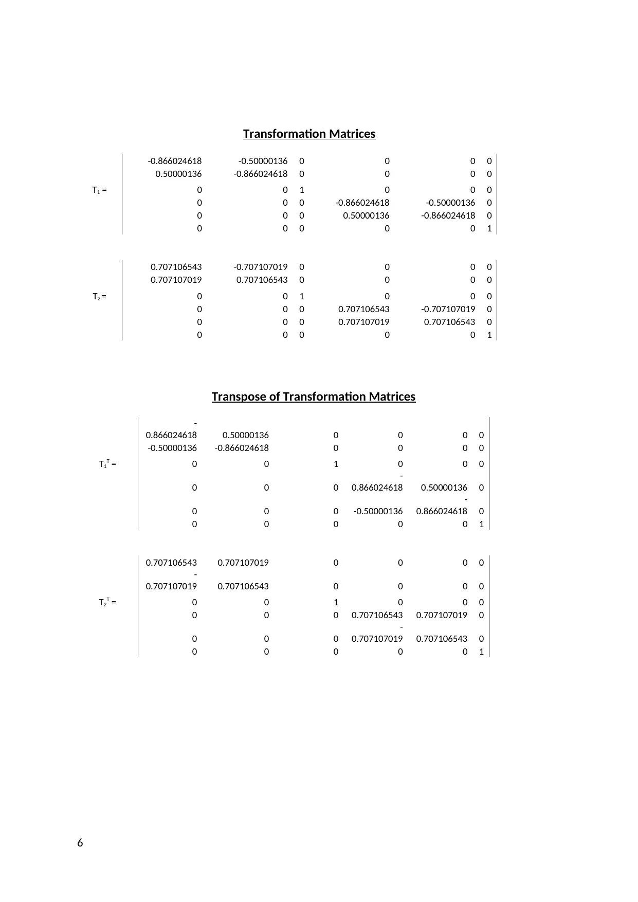
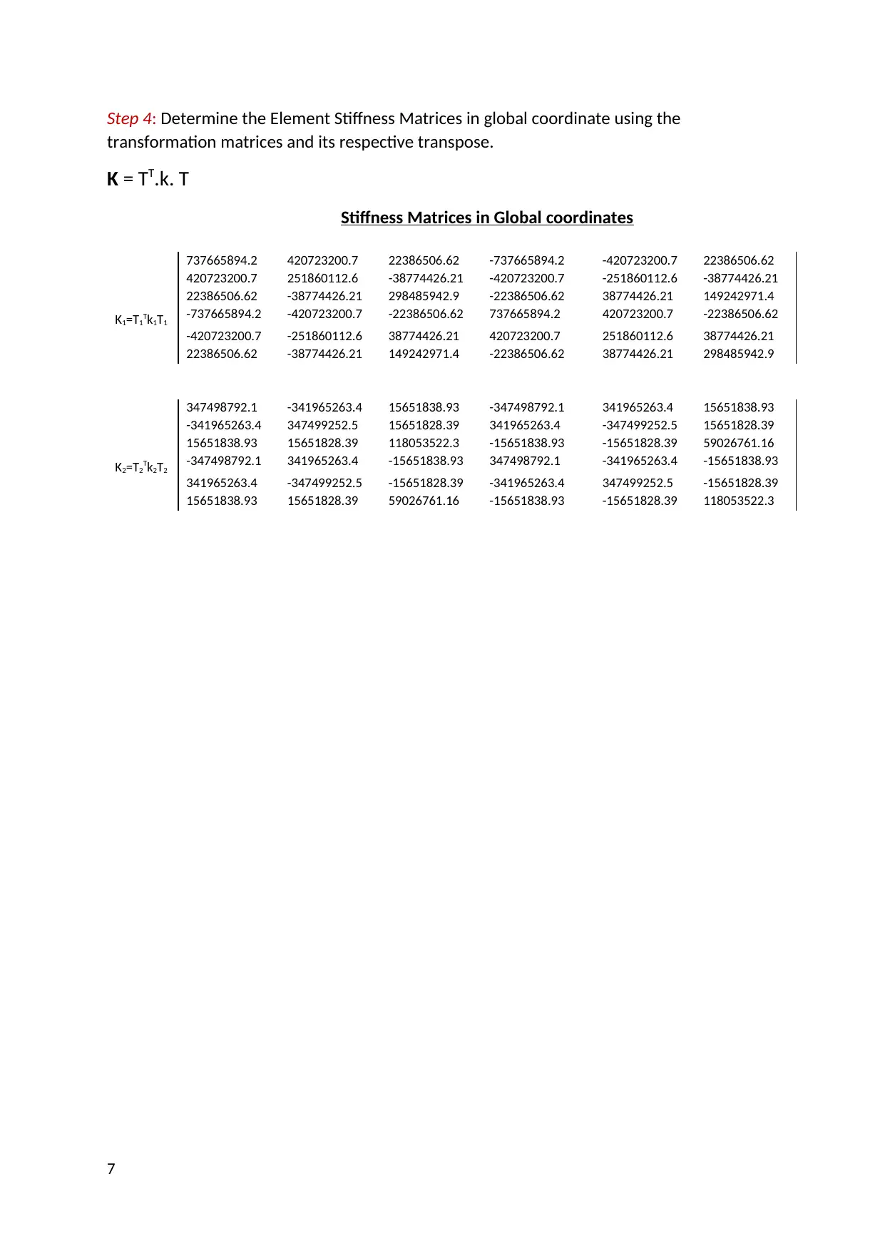
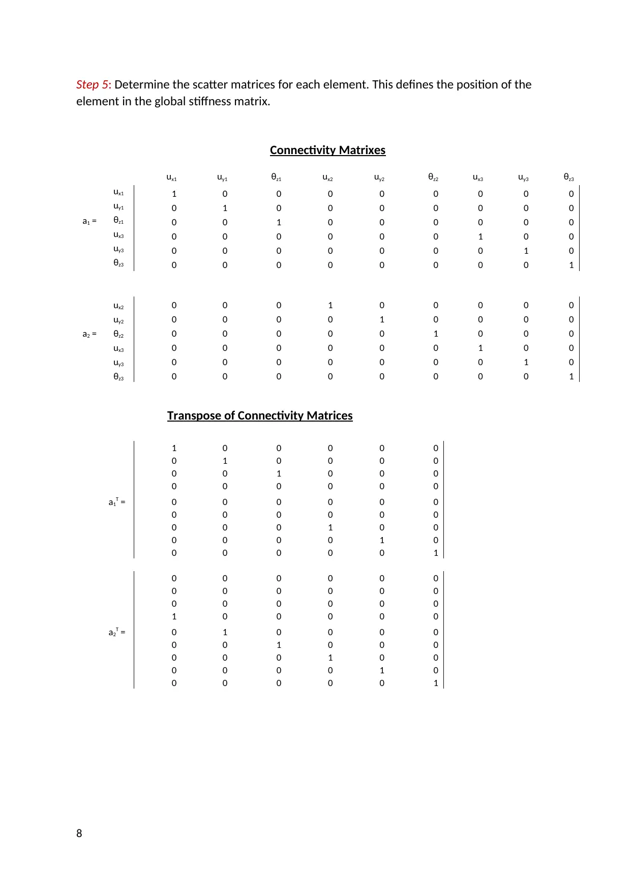
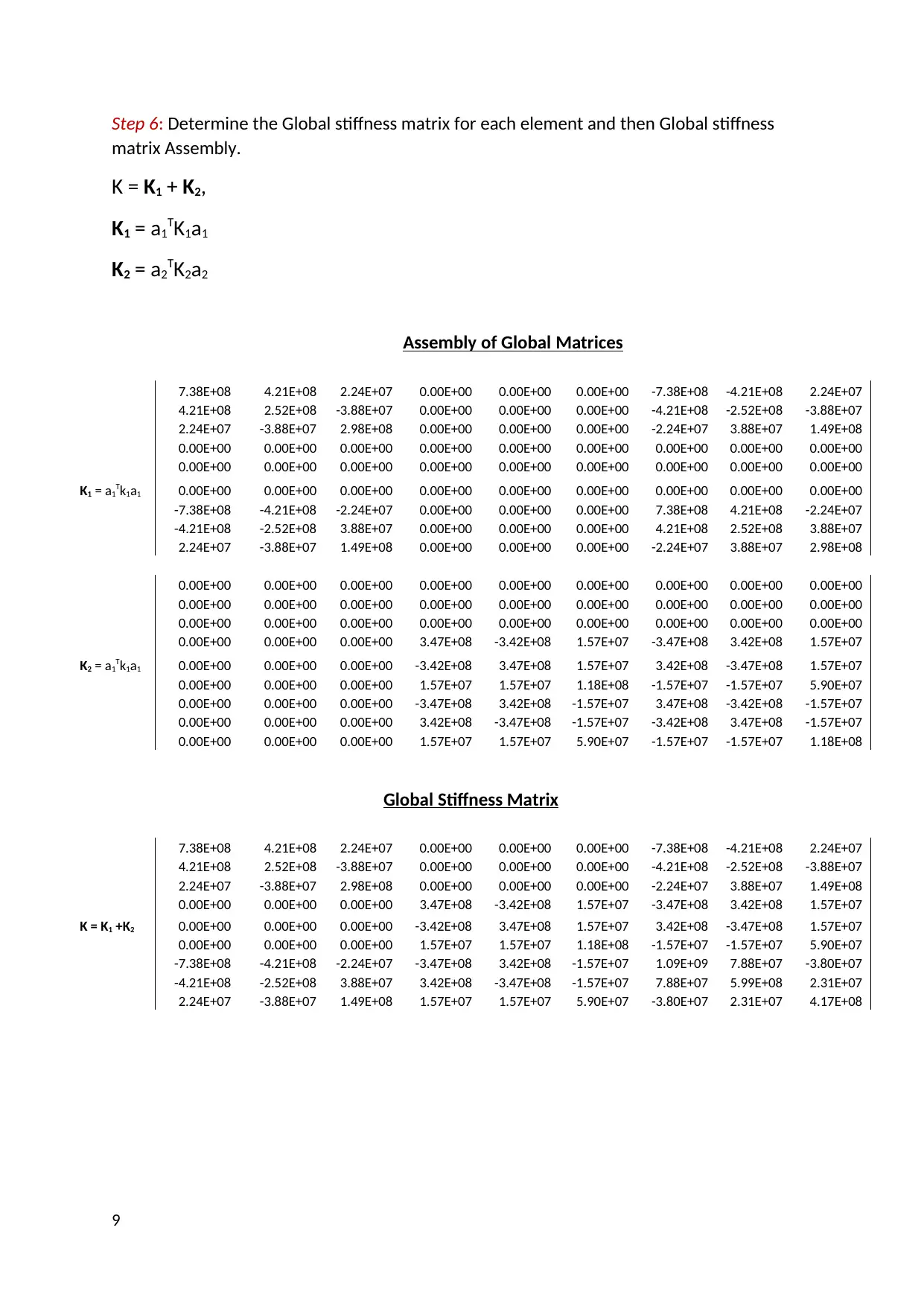
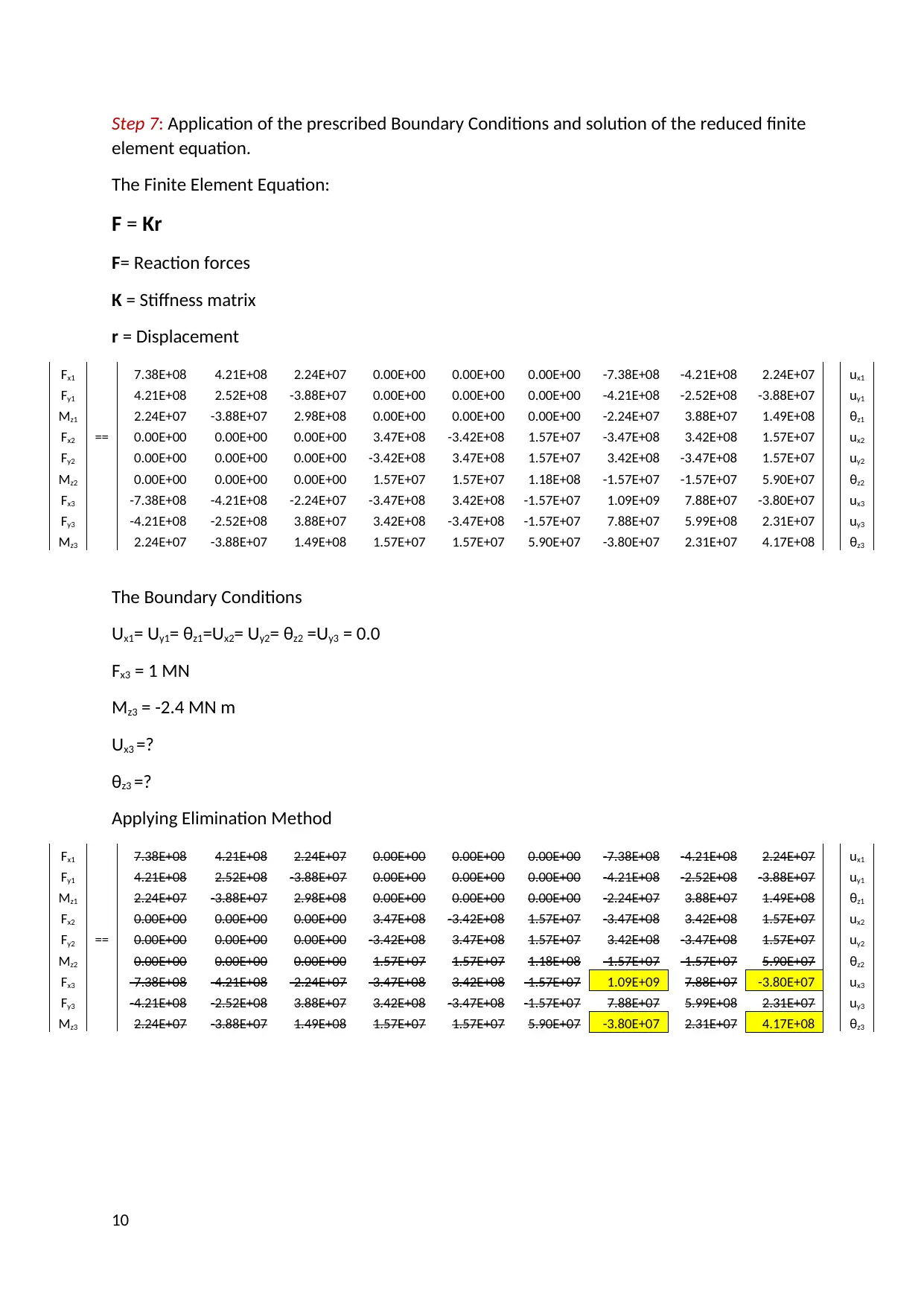
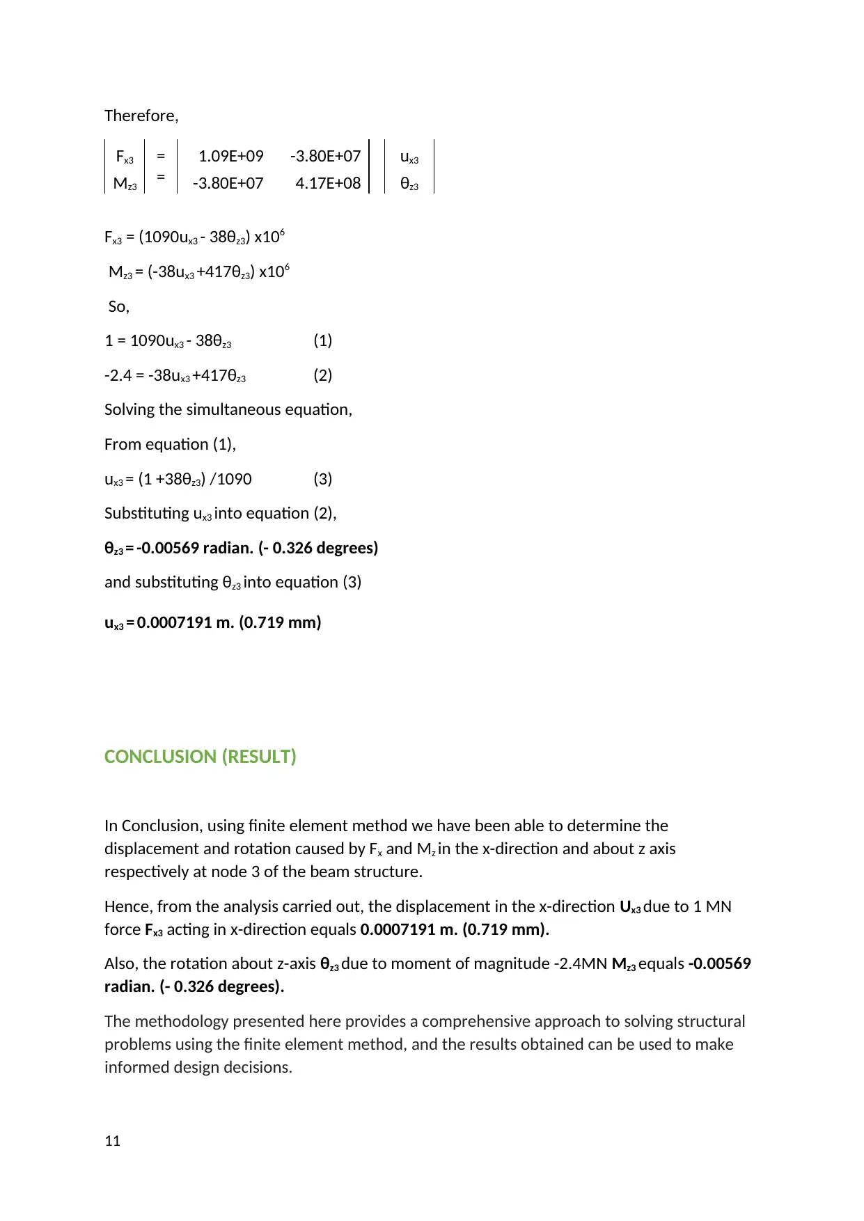
This document provides a comprehensive solution to a Finite Element Method (FEM) assignment, focusing on the analysis of a 2D beam structure. The assignment involves calculating the displacement in the x-direction and the rotation about the z-direction at a global node of the beam. The solution details the steps of the FEM, including discretization, determination of element stiffness matrices in local and global coordinates, transformation matrices, assembly of the global stiffness matrix, application of boundary conditions, and the determination of unknowns. The beam is discretized into two elements with given properties (Young's modulus, diameter, wall thickness, length), and the global stiffness matrix is constructed. The methodology includes calculating internal diameters, areas, and second moment of area. Transformation matrices are used to move the element from local coordinates to global coordinates. Boundary conditions are applied, and the final displacement and rotation are calculated using elimination method. The results show the displacement in the x-direction and the rotation about the z-axis at the node. The assignment showcases a detailed application of FEM for structural analysis.

Finite Element Method (Part 1)
EG55M1
Assignment One
Completed by Group 1
Group Members
ADELEKE OLUGBENGA
GANGADHARAN NAMITA
MINHAJ MD HABIBULLAH

INTRODUCTION
Finite Element Method is a numerical method used to analyse complex engineering
structures and systems. This is achieved by partitioning the structure into smaller simpler
parts or elements. This method gives approximation solutions to physical problems.
Using finite element analysis method, we can determine the stress, strain and deformation
in the structure. In this problem the type of finite element analysis systems used is linear
static structural capabilities which is a beam in the x-y plane with degrees of freedom 𝑢𝑥,
𝑢𝑦 and 𝜃𝑧 at each end.
The element properties are given, which are then used to construct global properties, and
after the boundary conditions are imposed, then the displacement in the x-direction and the
rotation about the z-direction are calculated.
These are the steps required to solve the problem using finite element method.
 Discretisation
 Determination of the local element characteristics
 Transformation of the element characteristics
 Assembly of the global element characteristics
 Application of the boundary conditions
 Determination of the unknowns from the finite element equation
2

AIM
The aim of this report is to calculate the displacement in the x-direction and the rotation
about the z-direction for global node A of the beam shown below, using all the information
provided.
Question.
The stiffness matrix of a 2D beam element (i.e., a beam in the x-y plane with degrees of
freedom 𝑢𝑥, 𝑢𝑦 and 𝜃𝑧 at each end) is shown below (note the symmetry about the
leading diagonal).
Use the element stiffness matrix to construct the global stiffness matrix. Note that the
member 1 and member 2 are fully fixed at one end.
In the figure member 1 is ∅800𝑚𝑚 × 20𝑤𝑡 × 10𝑚 long and member 2 is∅600𝑚𝑚 × 15𝑤𝑡
× 8𝑚 long. Neglect the shear deformation (i.e., Φ = 0). Young’s modulus is 200 GPa.
Calculate the displacement in the x-direction and the rotation about the z-direction for
global node A when 𝐹𝑥 = 1𝑀𝑁 and 𝑀𝑧 = −2.4 𝑀𝑁𝑚. The transformation matrix for
this problem is a matrix with the rotational degree of freedom at each node.
3

4

METHODOLOGY
The problem above is solved using finite element method.
Step 1: Model discretisation, connectivity and properties. The table below shows the nodes
that are associated to each element. It also shows the properties and local characteristics of
the elements.
Element Node
1
Node
2
Angle
(°)
Young
Modulus
(N/m2)
External
Diameter
(m)
Wall
thickness
(m)
Internal
Dia. (m)
Area
(m2)
Length
(m)
Second
Moment
Area (m4)
θ E Do wt. Di A L I
1 1 3 210 2.00E+11 0.8 0.02 0.76 0.049 10 0.0037311
2 2 3 -45 2.00E+11 0.6 0.015 0.57 0.028 8 0.0011805
Calculate the Internal Diameters (Di), Areas (A) and Second Moment Area (I) using these
formulars.
Di = Do -wt.
A = ( /4) (Dỻ o2-Di2)
I = ( /64) (Dỻ o4-Di4)
Step 2: Determine the Element Stiffness Matrix in local coordinates.
Stiffness Matrices in Local Coordinates
9.81E+08 0 0 -9.81E+08 0 0
0 8.95E+06 4.48E+07 0 -8.95E+06 4.48E+07
k1 = 0 4.48E+07 2.98E+08 0 -4.48E+07 1.49E+08
-9.81E+08 0 0 9.81E+08 0 0
0 -8.95E+06 -4.48E+07 0 8.95E+06 -4.48E+07
0 4.48E+07 1.49E+08 0 -4.48E+07 2.98E+08
6.89E+08 0 0 -6.89E+08 0 0
0 5.53E+06 2.21E+07 0 -5.53E+06 2.21E+07
k2 = 0 2.21E+07 1.18E+08 0 -2.21E+07 5.90E+07
-6.89E+08 0 0 6.89E+08 0 0
0 -5.53E+06 -2.21E+07 0 5.53E+06 -2.21E+07
0 2.21E+07 5.90E+07 0 -2.21E+07 1.18E+08
Step 3: Determine the Element Transformation Matrices, this moves the element from local
coordinate to global coordinated system.
5

Transformation Matrices
-0.866024618 -0.50000136 0 0 0 0
0.50000136 -0.866024618 0 0 0 0
T1 = 0 0 1 0 0 0
0 0 0 -0.866024618 -0.50000136 0
0 0 0 0.50000136 -0.866024618 0
0 0 0 0 0 1
0.707106543 -0.707107019 0 0 0 0
0.707107019 0.707106543 0 0 0 0
T2 = 0 0 1 0 0 0
0 0 0 0.707106543 -0.707107019 0
0 0 0 0.707107019 0.707106543 0
0 0 0 0 0 1
Transpose of Transformation Matrices
-
0.866024618 0.50000136 0 0 0 0
-0.50000136 -0.866024618 0 0 0 0
T1T = 0 0 1 0 0 0
0 0 0
-
0.866024618 0.50000136 0
0 0 0 -0.50000136
-
0.866024618 0
0 0 0 0 0 1
0.707106543 0.707107019 0 0 0 0
-
0.707107019 0.707106543 0 0 0 0
T2T = 0 0 1 0 0 0
0 0 0 0.707106543 0.707107019 0
0 0 0
-
0.707107019 0.707106543 0
0 0 0 0 0 1
6

Step 4: Determine the Element Stiffness Matrices in global coordinate using the
transformation matrices and its respective transpose.
K = TT.k. T
Stiffness Matrices in Global coordinates
737665894.2 420723200.7 22386506.62 -737665894.2 -420723200.7 22386506.62
420723200.7 251860112.6 -38774426.21 -420723200.7 -251860112.6 -38774426.21
22386506.62 -38774426.21 298485942.9 -22386506.62 38774426.21 149242971.4
K1=T1Tk1T1 -737665894.2 -420723200.7 -22386506.62 737665894.2 420723200.7 -22386506.62
-420723200.7 -251860112.6 38774426.21 420723200.7 251860112.6 38774426.21
22386506.62 -38774426.21 149242971.4 -22386506.62 38774426.21 298485942.9
347498792.1 -341965263.4 15651838.93 -347498792.1 341965263.4 15651838.93
-341965263.4 347499252.5 15651828.39 341965263.4 -347499252.5 15651828.39
15651838.93 15651828.39 118053522.3 -15651838.93 -15651828.39 59026761.16
K2=T2Tk2T2 -347498792.1 341965263.4 -15651838.93 347498792.1 -341965263.4 -15651838.93
341965263.4 -347499252.5 -15651828.39 -341965263.4 347499252.5 -15651828.39
15651838.93 15651828.39 59026761.16 -15651838.93 -15651828.39 118053522.3
7

Step 5: Determine the scatter matrices for each element. This defines the position of the
element in the global stiffness matrix.
Connectivity Matrixes
ux1 uy1 θz1 ux2 uy2 θz2 ux3 uy3 θz3
ux1 1 0 0 0 0 0 0 0 0
uy1 0 1 0 0 0 0 0 0 0
a1 = θz1 0 0 1 0 0 0 0 0 0
ux3 0 0 0 0 0 0 1 0 0
uy3 0 0 0 0 0 0 0 1 0
θz3 0 0 0 0 0 0 0 0 1
ux2 0 0 0 1 0 0 0 0 0
uy2 0 0 0 0 1 0 0 0 0
a2 = θz2 0 0 0 0 0 1 0 0 0
ux3 0 0 0 0 0 0 1 0 0
uy3 0 0 0 0 0 0 0 1 0
θz3 0 0 0 0 0 0 0 0 1
Transpose of Connectivity Matrices
1 0 0 0 0 0
0 1 0 0 0 0
0 0 1 0 0 0
0 0 0 0 0 0
a1T = 0 0 0 0 0 0
0 0 0 0 0 0
0 0 0 1 0 0
0 0 0 0 1 0
0 0 0 0 0 1
0 0 0 0 0 0
0 0 0 0 0 0
0 0 0 0 0 0
1 0 0 0 0 0
a2T = 0 1 0 0 0 0
0 0 1 0 0 0
0 0 0 1 0 0
0 0 0 0 1 0
0 0 0 0 0 1
8

Step 6: Determine the Global stiffness matrix for each element and then Global stiffness
matrix Assembly.
K = K1 + K2,
K1 = a1TK1a1
K2 = a2TK2a2
Assembly of Global Matrices
7.38E+08 4.21E+08 2.24E+07 0.00E+00 0.00E+00 0.00E+00 -7.38E+08 -4.21E+08 2.24E+07
4.21E+08 2.52E+08 -3.88E+07 0.00E+00 0.00E+00 0.00E+00 -4.21E+08 -2.52E+08 -3.88E+07
2.24E+07 -3.88E+07 2.98E+08 0.00E+00 0.00E+00 0.00E+00 -2.24E+07 3.88E+07 1.49E+08
0.00E+00 0.00E+00 0.00E+00 0.00E+00 0.00E+00 0.00E+00 0.00E+00 0.00E+00 0.00E+00
0.00E+00 0.00E+00 0.00E+00 0.00E+00 0.00E+00 0.00E+00 0.00E+00 0.00E+00 0.00E+00
K1 = a1Tk1a1 0.00E+00 0.00E+00 0.00E+00 0.00E+00 0.00E+00 0.00E+00 0.00E+00 0.00E+00 0.00E+00
-7.38E+08 -4.21E+08 -2.24E+07 0.00E+00 0.00E+00 0.00E+00 7.38E+08 4.21E+08 -2.24E+07
-4.21E+08 -2.52E+08 3.88E+07 0.00E+00 0.00E+00 0.00E+00 4.21E+08 2.52E+08 3.88E+07
2.24E+07 -3.88E+07 1.49E+08 0.00E+00 0.00E+00 0.00E+00 -2.24E+07 3.88E+07 2.98E+08
0.00E+00 0.00E+00 0.00E+00 0.00E+00 0.00E+00 0.00E+00 0.00E+00 0.00E+00 0.00E+00
0.00E+00 0.00E+00 0.00E+00 0.00E+00 0.00E+00 0.00E+00 0.00E+00 0.00E+00 0.00E+00
0.00E+00 0.00E+00 0.00E+00 0.00E+00 0.00E+00 0.00E+00 0.00E+00 0.00E+00 0.00E+00
0.00E+00 0.00E+00 0.00E+00 3.47E+08 -3.42E+08 1.57E+07 -3.47E+08 3.42E+08 1.57E+07
K2 = a1Tk1a1 0.00E+00 0.00E+00 0.00E+00 -3.42E+08 3.47E+08 1.57E+07 3.42E+08 -3.47E+08 1.57E+07
0.00E+00 0.00E+00 0.00E+00 1.57E+07 1.57E+07 1.18E+08 -1.57E+07 -1.57E+07 5.90E+07
0.00E+00 0.00E+00 0.00E+00 -3.47E+08 3.42E+08 -1.57E+07 3.47E+08 -3.42E+08 -1.57E+07
0.00E+00 0.00E+00 0.00E+00 3.42E+08 -3.47E+08 -1.57E+07 -3.42E+08 3.47E+08 -1.57E+07
0.00E+00 0.00E+00 0.00E+00 1.57E+07 1.57E+07 5.90E+07 -1.57E+07 -1.57E+07 1.18E+08
Global Stiffness Matrix
7.38E+08 4.21E+08 2.24E+07 0.00E+00 0.00E+00 0.00E+00 -7.38E+08 -4.21E+08 2.24E+07
4.21E+08 2.52E+08 -3.88E+07 0.00E+00 0.00E+00 0.00E+00 -4.21E+08 -2.52E+08 -3.88E+07
2.24E+07 -3.88E+07 2.98E+08 0.00E+00 0.00E+00 0.00E+00 -2.24E+07 3.88E+07 1.49E+08
0.00E+00 0.00E+00 0.00E+00 3.47E+08 -3.42E+08 1.57E+07 -3.47E+08 3.42E+08 1.57E+07
K = K1 +K2 0.00E+00 0.00E+00 0.00E+00 -3.42E+08 3.47E+08 1.57E+07 3.42E+08 -3.47E+08 1.57E+07
0.00E+00 0.00E+00 0.00E+00 1.57E+07 1.57E+07 1.18E+08 -1.57E+07 -1.57E+07 5.90E+07
-7.38E+08 -4.21E+08 -2.24E+07 -3.47E+08 3.42E+08 -1.57E+07 1.09E+09 7.88E+07 -3.80E+07
-4.21E+08 -2.52E+08 3.88E+07 3.42E+08 -3.47E+08 -1.57E+07 7.88E+07 5.99E+08 2.31E+07
2.24E+07 -3.88E+07 1.49E+08 1.57E+07 1.57E+07 5.90E+07 -3.80E+07 2.31E+07 4.17E+08
9

Step 7: Application of the prescribed Boundary Conditions and solution of the reduced finite
element equation.
The Finite Element Equation:
F = Kr
F= Reaction forces
K = Stiffness matrix
r = Displacement
Fx1 7.38E+08 4.21E+08 2.24E+07 0.00E+00 0.00E+00 0.00E+00 -7.38E+08 -4.21E+08 2.24E+07 ux1
Fy1 4.21E+08 2.52E+08 -3.88E+07 0.00E+00 0.00E+00 0.00E+00 -4.21E+08 -2.52E+08 -3.88E+07 uy1
Mz1 2.24E+07 -3.88E+07 2.98E+08 0.00E+00 0.00E+00 0.00E+00 -2.24E+07 3.88E+07 1.49E+08 θz1
Fx2 == 0.00E+00 0.00E+00 0.00E+00 3.47E+08 -3.42E+08 1.57E+07 -3.47E+08 3.42E+08 1.57E+07 ux2
Fy2 0.00E+00 0.00E+00 0.00E+00 -3.42E+08 3.47E+08 1.57E+07 3.42E+08 -3.47E+08 1.57E+07 uy2
Mz2 0.00E+00 0.00E+00 0.00E+00 1.57E+07 1.57E+07 1.18E+08 -1.57E+07 -1.57E+07 5.90E+07 θz2
Fx3 -7.38E+08 -4.21E+08 -2.24E+07 -3.47E+08 3.42E+08 -1.57E+07 1.09E+09 7.88E+07 -3.80E+07 ux3
Fy3 -4.21E+08 -2.52E+08 3.88E+07 3.42E+08 -3.47E+08 -1.57E+07 7.88E+07 5.99E+08 2.31E+07 uy3
Mz3 2.24E+07 -3.88E+07 1.49E+08 1.57E+07 1.57E+07 5.90E+07 -3.80E+07 2.31E+07 4.17E+08 θz3
The Boundary Conditions
Ux1= Uy1= θz1=Ux2= Uy2= θz2 =Uy3 = 0.0
Fx3 = 1 MN
Mz3 = -2.4 MN m
Ux3 =?
θz3 =?
Applying Elimination Method
Fx1 7.38E+08 4.21E+08 2.24E+07 0.00E+00 0.00E+00 0.00E+00 -7.38E+08 -4.21E+08 2.24E+07 ux1
Fy1 4.21E+08 2.52E+08 -3.88E+07 0.00E+00 0.00E+00 0.00E+00 -4.21E+08 -2.52E+08 -3.88E+07 uy1
Mz1 2.24E+07 -3.88E+07 2.98E+08 0.00E+00 0.00E+00 0.00E+00 -2.24E+07 3.88E+07 1.49E+08 θz1
Fx2 0.00E+00 0.00E+00 0.00E+00 3.47E+08 -3.42E+08 1.57E+07 -3.47E+08 3.42E+08 1.57E+07 ux2
Fy2 == 0.00E+00 0.00E+00 0.00E+00 -3.42E+08 3.47E+08 1.57E+07 3.42E+08 -3.47E+08 1.57E+07 uy2
Mz2 0.00E+00 0.00E+00 0.00E+00 1.57E+07 1.57E+07 1.18E+08 -1.57E+07 -1.57E+07 5.90E+07 θz2
Fx3 -7.38E+08 -4.21E+08 -2.24E+07 -3.47E+08 3.42E+08 -1.57E+07 1.09E+09 7.88E+07 -3.80E+07 ux3
Fy3 -4.21E+08 -2.52E+08 3.88E+07 3.42E+08 -3.47E+08 -1.57E+07 7.88E+07 5.99E+08 2.31E+07 uy3
Mz3 2.24E+07 -3.88E+07 1.49E+08 1.57E+07 1.57E+07 5.90E+07 -3.80E+07 2.31E+07 4.17E+08 θz3
10

Therefore,
Fx3 =
=
1.09E+09 -3.80E+07 ux3
Mz3 -3.80E+07 4.17E+08 θz3
Fx3 = (1090ux3 - 38θz3) x106
Mz3 = (-38ux3 +417θz3) x106
So,
1 = 1090ux3 - 38θz3 (1)
-2.4 = -38ux3 +417θz3 (2)
Solving the simultaneous equation,
From equation (1),
ux3 = (1 +38θz3) /1090 (3)
Substituting ux3 into equation (2),
θz3 = -0.00569 radian. (- 0.326 degrees)
and substituting θz3 into equation (3)
ux3 = 0.0007191 m. (0.719 mm)
CONCLUSION (RESULT)
In Conclusion, using finite element method we have been able to determine the
displacement and rotation caused by Fx and Mz in the x-direction and about z axis
respectively at node 3 of the beam structure.
Hence, from the analysis carried out, the displacement in the x-direction Ux3 due to 1 MN
force Fx3 acting in x-direction equals 0.0007191 m. (0.719 mm).
Also, the rotation about z-axis θz3 due to moment of magnitude -2.4MN Mz3 equals -0.00569
radian. (- 0.326 degrees).
The methodology presented here provides a comprehensive approach to solving structural
problems using the finite element method, and the results obtained can be used to make
informed design decisions.
11