FIN10002: Statistical Analysis and Report on Australian Sales Data
VerifiedAdded on 2023/06/15
|20
|2987
|306
Homework Assignment
AI Summary
This assignment provides a comprehensive financial statistics analysis of Australian sales data, encompassing descriptive statistics for quantitative variables and graphical representations for qualitative variables. It includes the calculation and interpretation of confidence intervals for sales and shipping costs, hypothesis testing to compare shipping costs based on order priority and average sales across different regions, and a linear regression analysis to assess the relationship between sales and order quantity. The analysis reveals key insights into order patterns, shipping costs, regional sales variations, and the limited linear association between sales and order quantity. Desklib offers a platform to access this and many more solved assignments.
Running head: FINANCIAL STATISTICS
Financial Statistics
Name of the Student:
Name of the University:
Author’s note:
Financial Statistics
Name of the Student:
Name of the University:
Author’s note:
Paraphrase This Document
Need a fresh take? Get an instant paraphrase of this document with our AI Paraphraser
1FINANCIAL STATISTICS
Table of Contents
Tasks..........................................................................................................................................3
Task 1:....................................................................................................................................3
Task 2:....................................................................................................................................3
Quantitative Variables:.......................................................................................................3
Qualitative Variables:.........................................................................................................5
Task 3 – Confidence Interval:................................................................................................9
Task 3.1..............................................................................................................................9
Task 3.2............................................................................................................................10
Task 4 – Hypothesis Testing:...............................................................................................10
Task 4.1............................................................................................................................10
Task 4.2............................................................................................................................11
Task 5 – Correlation and regression:...................................................................................12
Task 5.1................................................................................................................................12
Task 5.2................................................................................................................................13
Task 5.3................................................................................................................................13
Task 5.4................................................................................................................................13
Conclusion:..............................................................................................................................14
References:...............................................................................................................................15
Appendices:..............................................................................................................................16
Task 3 – Confidence Interval:..............................................................................................16
2FINANCIAL STATISTICS
Task 4 – Hypothesis Testing:...............................................................................................16
Task 5 – Correlation and regression:...................................................................................17
Task 4 – Hypothesis Testing:...............................................................................................16
Task 5 – Correlation and regression:...................................................................................17
⊘ This is a preview!⊘
Do you want full access?
Subscribe today to unlock all pages.
Trusted by 1+ million students worldwide
3FINANCIAL STATISTICS
Tasks
Task 1:
The selected 60 random variables out of 2002 random variables are collected. The
option “Random Variable Generation” of “Data Analysis” toolpack is used for extracting
random variable.
Task 2:
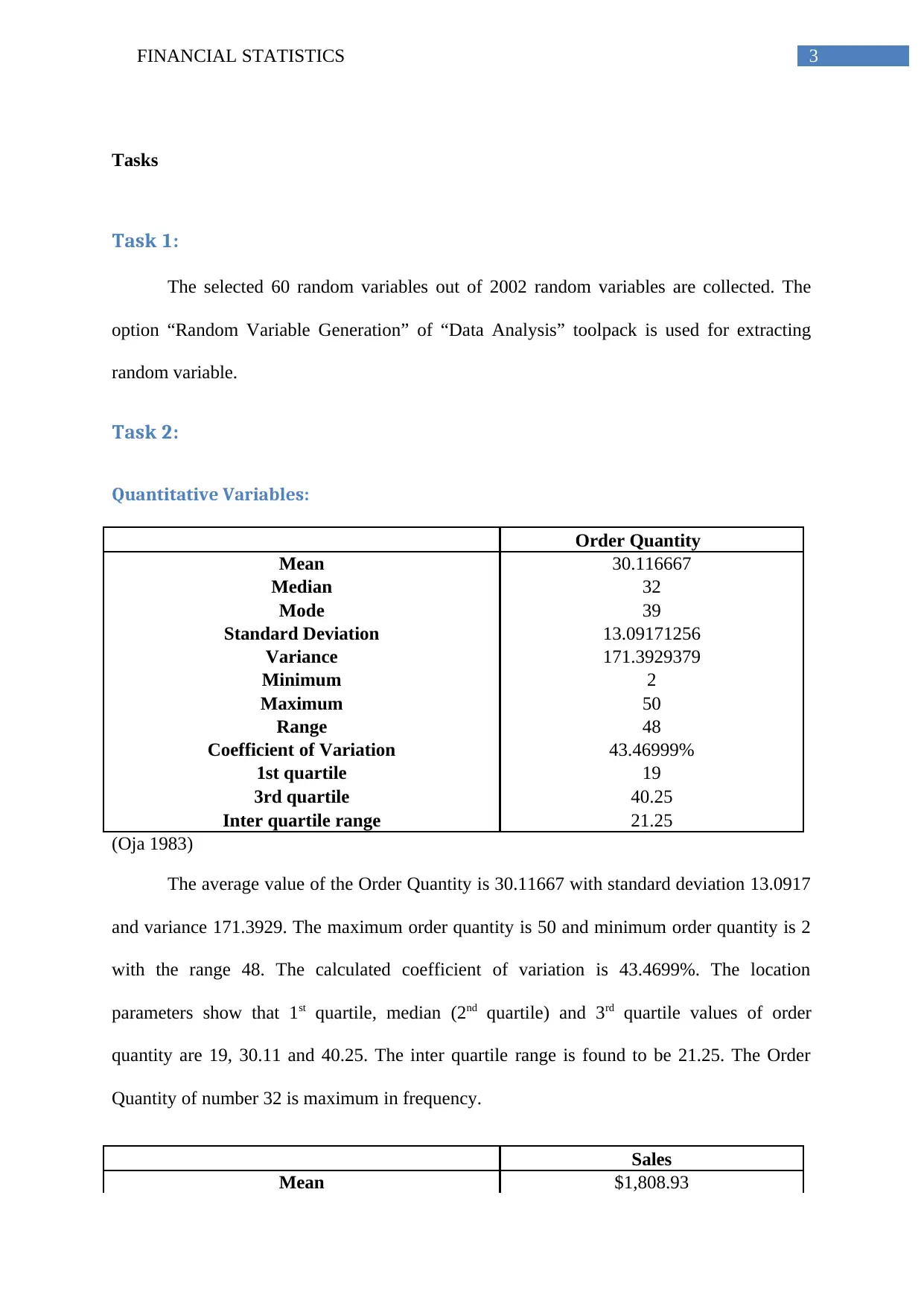
Quantitative Variables:
Order Quantity
Mean 30.116667
Median 32
Mode 39
Standard Deviation 13.09171256
Variance 171.3929379
Minimum 2
Maximum 50
Range 48
Coefficient of Variation 43.46999%
1st quartile 19
3rd quartile 40.25
Inter quartile range 21.25
(Oja 1983)
The average value of the Order Quantity is 30.11667 with standard deviation 13.0917
and variance 171.3929. The maximum order quantity is 50 and minimum order quantity is 2
with the range 48. The calculated coefficient of variation is 43.4699%. The location
parameters show that 1st quartile, median (2nd quartile) and 3rd quartile values of order
quantity are 19, 30.11 and 40.25. The inter quartile range is found to be 21.25. The Order
Quantity of number 32 is maximum in frequency.
Sales
Mean $1,808.93
Tasks
Task 1:
The selected 60 random variables out of 2002 random variables are collected. The
option “Random Variable Generation” of “Data Analysis” toolpack is used for extracting
random variable.
Task 2:
Quantitative Variables:
Order Quantity
Mean 30.116667
Median 32
Mode 39
Standard Deviation 13.09171256
Variance 171.3929379
Minimum 2
Maximum 50
Range 48
Coefficient of Variation 43.46999%
1st quartile 19
3rd quartile 40.25
Inter quartile range 21.25
(Oja 1983)
The average value of the Order Quantity is 30.11667 with standard deviation 13.0917
and variance 171.3929. The maximum order quantity is 50 and minimum order quantity is 2
with the range 48. The calculated coefficient of variation is 43.4699%. The location
parameters show that 1st quartile, median (2nd quartile) and 3rd quartile values of order
quantity are 19, 30.11 and 40.25. The inter quartile range is found to be 21.25. The Order
Quantity of number 32 is maximum in frequency.
Sales
Mean $1,808.93
Paraphrase This Document
Need a fresh take? Get an instant paraphrase of this document with our AI Paraphraser
4FINANCIAL STATISTICS
Median $579.59
Mode #N/A
Standard Deviation $3,340.82
Variance $11,161,055.62
Minimum $30.10
Maximum $18,056.68
Range $18,026.58
Coefficient of Variation 184.68425%
1st quartile $185.93
3rd quartile $1,711.22
Inter quartile range $1,525.29
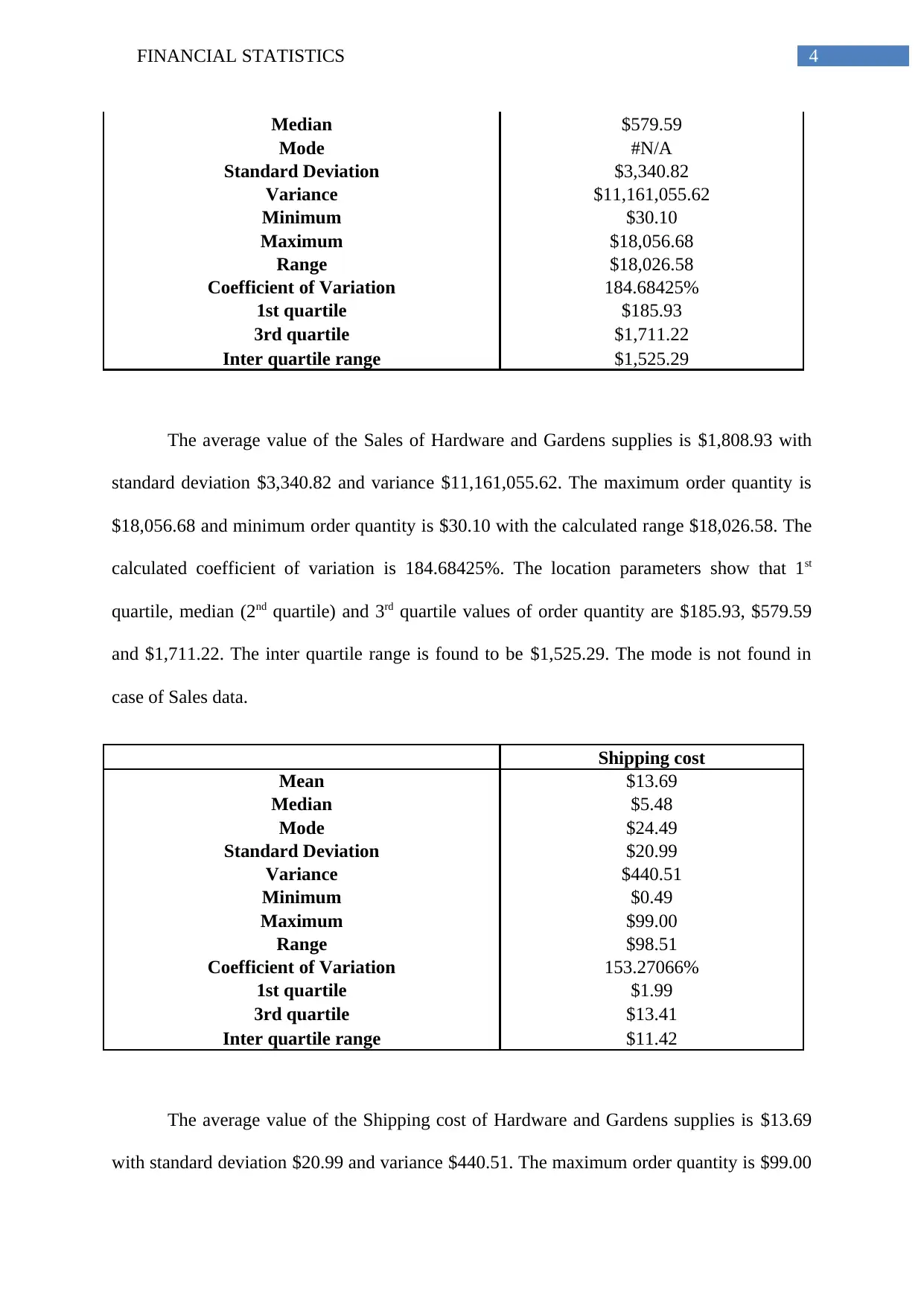
The average value of the Sales of Hardware and Gardens supplies is $1,808.93 with
standard deviation $3,340.82 and variance $11,161,055.62. The maximum order quantity is
$18,056.68 and minimum order quantity is $30.10 with the calculated range $18,026.58. The
calculated coefficient of variation is 184.68425%. The location parameters show that 1st
quartile, median (2nd quartile) and 3rd quartile values of order quantity are $185.93, $579.59
and $1,711.22. The inter quartile range is found to be $1,525.29. The mode is not found in
case of Sales data.
Shipping cost
Mean $13.69
Median $5.48
Mode $24.49
Standard Deviation $20.99
Variance $440.51
Minimum $0.49
Maximum $99.00
Range $98.51
Coefficient of Variation 153.27066%
1st quartile $1.99
3rd quartile $13.41
Inter quartile range $11.42
The average value of the Shipping cost of Hardware and Gardens supplies is $13.69
with standard deviation $20.99 and variance $440.51. The maximum order quantity is $99.00
Median $579.59
Mode #N/A
Standard Deviation $3,340.82
Variance $11,161,055.62
Minimum $30.10
Maximum $18,056.68
Range $18,026.58
Coefficient of Variation 184.68425%
1st quartile $185.93
3rd quartile $1,711.22
Inter quartile range $1,525.29
The average value of the Sales of Hardware and Gardens supplies is $1,808.93 with
standard deviation $3,340.82 and variance $11,161,055.62. The maximum order quantity is
$18,056.68 and minimum order quantity is $30.10 with the calculated range $18,026.58. The
calculated coefficient of variation is 184.68425%. The location parameters show that 1st
quartile, median (2nd quartile) and 3rd quartile values of order quantity are $185.93, $579.59
and $1,711.22. The inter quartile range is found to be $1,525.29. The mode is not found in
case of Sales data.
Shipping cost
Mean $13.69
Median $5.48
Mode $24.49
Standard Deviation $20.99
Variance $440.51
Minimum $0.49
Maximum $99.00
Range $98.51
Coefficient of Variation 153.27066%
1st quartile $1.99
3rd quartile $13.41
Inter quartile range $11.42
The average value of the Shipping cost of Hardware and Gardens supplies is $13.69
with standard deviation $20.99 and variance $440.51. The maximum order quantity is $99.00
5FINANCIAL STATISTICS
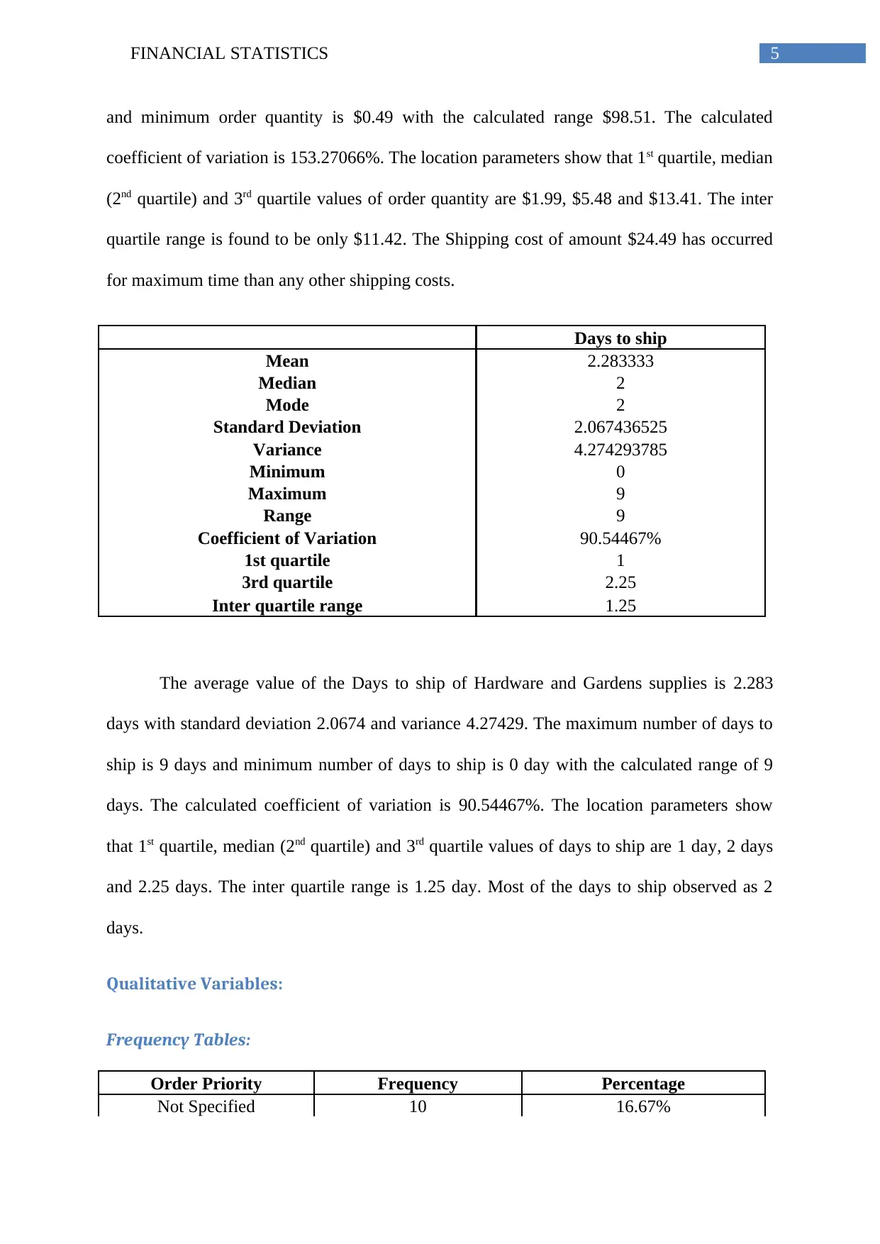
and minimum order quantity is $0.49 with the calculated range $98.51. The calculated
coefficient of variation is 153.27066%. The location parameters show that 1st quartile, median
(2nd quartile) and 3rd quartile values of order quantity are $1.99, $5.48 and $13.41. The inter
quartile range is found to be only $11.42. The Shipping cost of amount $24.49 has occurred
for maximum time than any other shipping costs.
Days to ship
Mean 2.283333
Median 2
Mode 2
Standard Deviation 2.067436525
Variance 4.274293785
Minimum 0
Maximum 9
Range 9
Coefficient of Variation 90.54467%
1st quartile 1
3rd quartile 2.25
Inter quartile range 1.25
The average value of the Days to ship of Hardware and Gardens supplies is 2.283
days with standard deviation 2.0674 and variance 4.27429. The maximum number of days to
ship is 9 days and minimum number of days to ship is 0 day with the calculated range of 9
days. The calculated coefficient of variation is 90.54467%. The location parameters show
that 1st quartile, median (2nd quartile) and 3rd quartile values of days to ship are 1 day, 2 days
and 2.25 days. The inter quartile range is 1.25 day. Most of the days to ship observed as 2
days.
Qualitative Variables:
Frequency Tables:
Order Priority Frequency Percentage
Not Specified 10 16.67%
⊘ This is a preview!⊘
Do you want full access?
Subscribe today to unlock all pages.
Trusted by 1+ million students worldwide
6FINANCIAL STATISTICS
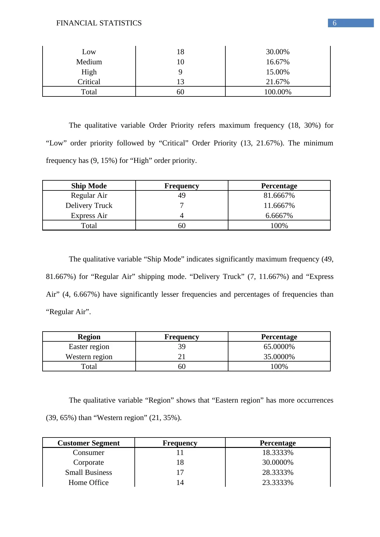
Low 18 30.00%
Medium 10 16.67%
High 9 15.00%
Critical 13 21.67%
Total 60 100.00%
The qualitative variable Order Priority refers maximum frequency (18, 30%) for
“Low” order priority followed by “Critical” Order Priority (13, 21.67%). The minimum
frequency has (9, 15%) for “High” order priority.
Ship Mode Frequency Percentage
Regular Air 49 81.6667%
Delivery Truck 7 11.6667%
Express Air 4 6.6667%
Total 60 100%
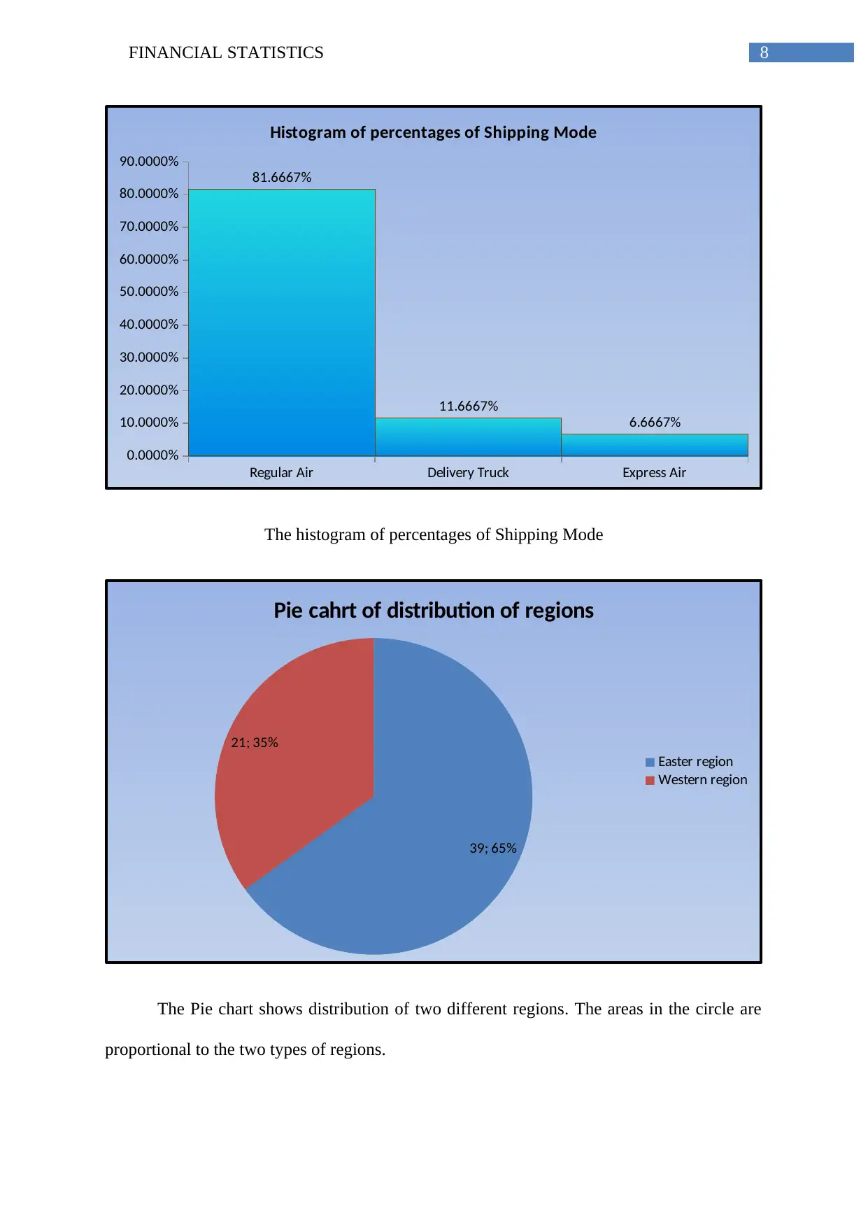
The qualitative variable “Ship Mode” indicates significantly maximum frequency (49,
81.667%) for “Regular Air” shipping mode. “Delivery Truck” (7, 11.667%) and “Express
Air” (4, 6.667%) have significantly lesser frequencies and percentages of frequencies than
“Regular Air”.
Region Frequency Percentage
Easter region 39 65.0000%
Western region 21 35.0000%
Total 60 100%
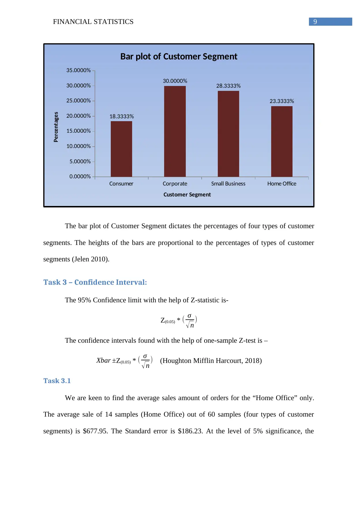
The qualitative variable “Region” shows that “Eastern region” has more occurrences
(39, 65%) than “Western region” (21, 35%).
Customer Segment Frequency Percentage
Consumer 11 18.3333%
Corporate 18 30.0000%
Small Business 17 28.3333%
Home Office 14 23.3333%
Low 18 30.00%
Medium 10 16.67%
High 9 15.00%
Critical 13 21.67%
Total 60 100.00%
The qualitative variable Order Priority refers maximum frequency (18, 30%) for
“Low” order priority followed by “Critical” Order Priority (13, 21.67%). The minimum
frequency has (9, 15%) for “High” order priority.
Ship Mode Frequency Percentage
Regular Air 49 81.6667%
Delivery Truck 7 11.6667%
Express Air 4 6.6667%
Total 60 100%
The qualitative variable “Ship Mode” indicates significantly maximum frequency (49,
81.667%) for “Regular Air” shipping mode. “Delivery Truck” (7, 11.667%) and “Express
Air” (4, 6.667%) have significantly lesser frequencies and percentages of frequencies than
“Regular Air”.
Region Frequency Percentage
Easter region 39 65.0000%
Western region 21 35.0000%
Total 60 100%
The qualitative variable “Region” shows that “Eastern region” has more occurrences
(39, 65%) than “Western region” (21, 35%).
Customer Segment Frequency Percentage
Consumer 11 18.3333%
Corporate 18 30.0000%
Small Business 17 28.3333%
Home Office 14 23.3333%
Paraphrase This Document
Need a fresh take? Get an instant paraphrase of this document with our AI Paraphraser
7FINANCIAL STATISTICS
Total 60 100.0000%
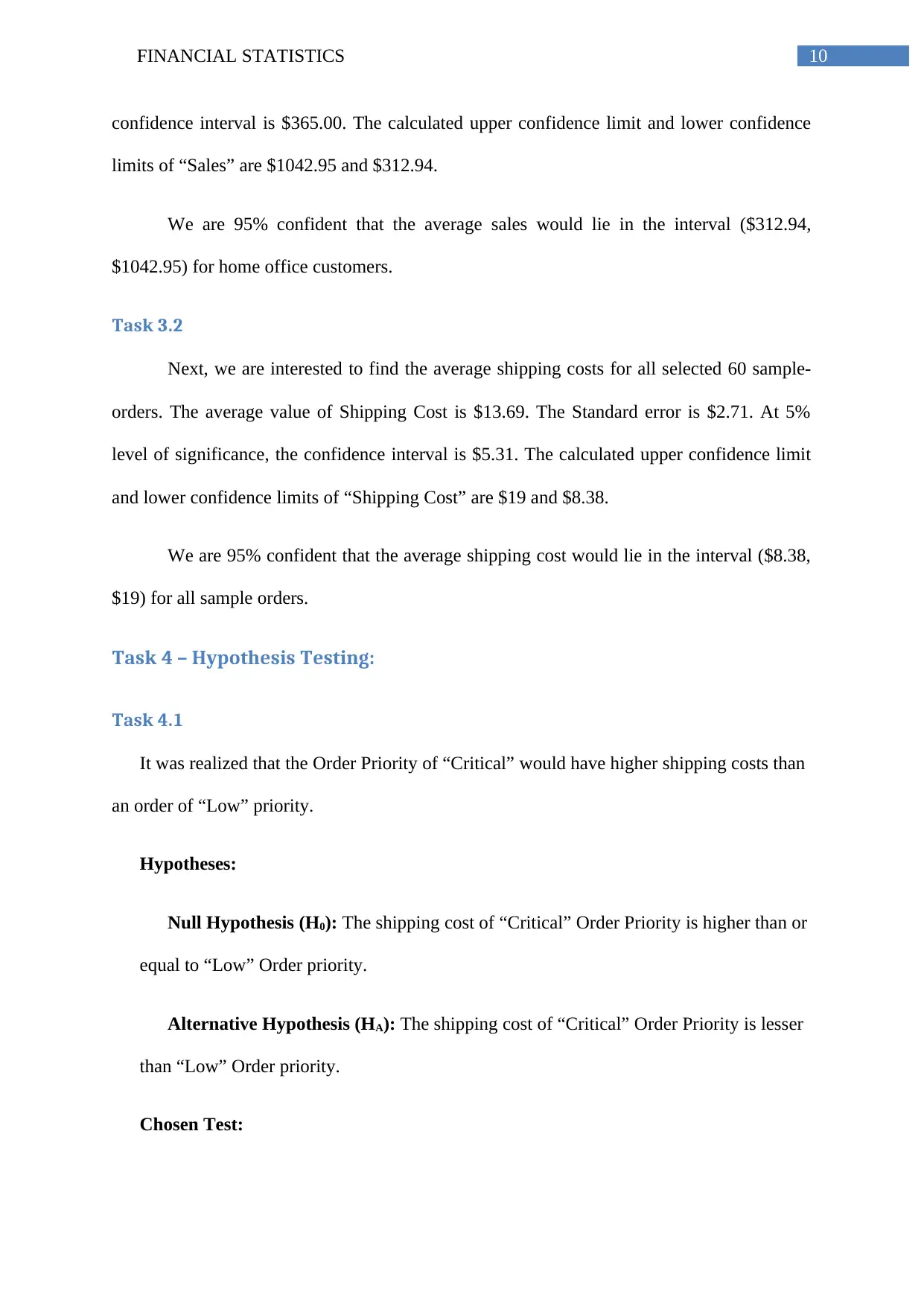
The “Customer Segment” refers that most of the customers are working in
“Corporate” with frequency 18 and percentage 30% followed by “Small Business” with
frequency 17 and percentage 28.33%. The minimum Customer Segment is observed in
“Corporate” (11, 18.33%).
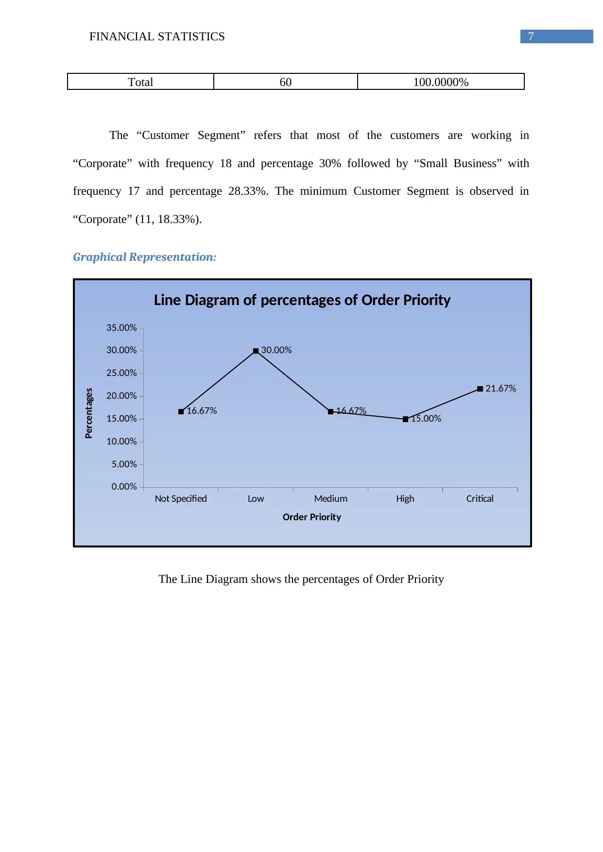
Graphical Representation:
Not Specified Low Medium High Critical
0.00%
5.00%
10.00%
15.00%
20.00%
25.00%
30.00%
35.00%
16.67%
30.00%
16.67% 15.00%
21.67%
Line Diagram of percentages of Order Priority
Order Priority
Percentages
The Line Diagram shows the percentages of Order Priority
Total 60 100.0000%
The “Customer Segment” refers that most of the customers are working in
“Corporate” with frequency 18 and percentage 30% followed by “Small Business” with
frequency 17 and percentage 28.33%. The minimum Customer Segment is observed in
“Corporate” (11, 18.33%).
Graphical Representation:
Not Specified Low Medium High Critical
0.00%
5.00%
10.00%
15.00%
20.00%
25.00%
30.00%
35.00%
16.67%
30.00%
16.67% 15.00%
21.67%
Line Diagram of percentages of Order Priority
Order Priority
Percentages
The Line Diagram shows the percentages of Order Priority
8FINANCIAL STATISTICS
Regular Air Delivery Truck Express Air
0.0000%
10.0000%
20.0000%
30.0000%
40.0000%
50.0000%
60.0000%
70.0000%
80.0000%
90.0000%
81.6667%
11.6667%
6.6667%
Histogram of percentages of Shipping Mode
The histogram of percentages of Shipping Mode
39; 65%
21; 35%
Pie cahrt of distribution of regions
Easter region
Western region
The Pie chart shows distribution of two different regions. The areas in the circle are
proportional to the two types of regions.
⊘ This is a preview!⊘
Do you want full access?
Subscribe today to unlock all pages.
Trusted by 1+ million students worldwide
9FINANCIAL STATISTICS
Consumer Corporate Small Business Home Office
0.0000%
5.0000%
10.0000%
15.0000%
20.0000%
25.0000%
30.0000%
35.0000%
18.3333%
30.0000% 28.3333%
23.3333%
Bar plot of Customer Segment
Customer Segment
Percentages
The bar plot of Customer Segment dictates the percentages of four types of customer
segments. The heights of the bars are proportional to the percentages of types of customer
segments (Jelen 2010).
Task 3 – Confidence Interval:
The 95% Confidence limit with the help of Z-statistic is-
Z(0.05) * ( σ
√n )
The confidence intervals found with the help of one-sample Z-test is –
Xbar ±Z(0.05) * ( σ
√ n ) (Houghton Mifflin Harcourt, 2018)
Task 3.1
We are keen to find the average sales amount of orders for the “Home Office” only.
The average sale of 14 samples (Home Office) out of 60 samples (four types of customer
segments) is $677.95. The Standard error is $186.23. At the level of 5% significance, the
Paraphrase This Document
Need a fresh take? Get an instant paraphrase of this document with our AI Paraphraser
10FINANCIAL STATISTICS
confidence interval is $365.00. The calculated upper confidence limit and lower confidence
limits of “Sales” are $1042.95 and $312.94.
We are 95% confident that the average sales would lie in the interval ($312.94,
$1042.95) for home office customers.
Task 3.2
Next, we are interested to find the average shipping costs for all selected 60 sample-
orders. The average value of Shipping Cost is $13.69. The Standard error is $2.71. At 5%
level of significance, the confidence interval is $5.31. The calculated upper confidence limit
and lower confidence limits of “Shipping Cost” are $19 and $8.38.
We are 95% confident that the average shipping cost would lie in the interval ($8.38,
$19) for all sample orders.
Task 4 – Hypothesis Testing:
Task 4.1
It was realized that the Order Priority of “Critical” would have higher shipping costs than
an order of “Low” priority.
Hypotheses:
Null Hypothesis (H0): The shipping cost of “Critical” Order Priority is higher than or
equal to “Low” Order priority.
Alternative Hypothesis (HA): The shipping cost of “Critical” Order Priority is lesser
than “Low” Order priority.
Chosen Test:
11FINANCIAL STATISTICS
A Two-sample Z-test for equality of means is incorporated here for shipping costs of
two types of Order priority.
Level of Significance:
α=0.05
Inferential Statistic:
The Z-statistic is - z = ¿ ¿,
where,
x1bar and x2bar are two observed means.
μ1 and μ2 are two observed hypothetical averages.
n1 and n2 are numbers of two samples.
σ1 and σ2 are observed standard deviations of two samples.
The calculated Z-score for means of two samples is 0.53116.
p-Value:
The two-tail p-value for 95% confidence interval is 0.5953.
Conclusion:
Therefore, we accept the null hypothesis of greater or equality of shipping cost for
“Critical” Order Priority than “Low” Order Priority with 95% probability (Gardner and
Altman 1986).
Task 4.2
It is often felt that the mean values of order of sales in dollars, differs for Eastern states
(E) and Western states (W).
⊘ This is a preview!⊘
Do you want full access?
Subscribe today to unlock all pages.
Trusted by 1+ million students worldwide
1 out of 20
Related Documents


Your All-in-One AI-Powered Toolkit for Academic Success.
+13062052269
info@desklib.com
Available 24*7 on WhatsApp / Email
![[object Object]](/_next/static/media/star-bottom.7253800d.svg)
Unlock your academic potential
Copyright © 2020–2026 A2Z Services. All Rights Reserved. Developed and managed by ZUCOL.