FIN200 - Security Market Line, Capital Market Line & CAPM Analysis
VerifiedAdded on 2023/06/04
|11
|2573
|269
Report
AI Summary
This report provides a comparative analysis of the Security Market Line (SML) and Capital Market Line (CML), highlighting their differences using graphs and discussing the importance of minimum variance portfolios for investors. It examines how the beta coefficient and standard deviation are used to measure risk in SML and CML, respectively, and contrasts their approaches to portfolio efficiency. The report also explores the relevance of the Capital Asset Pricing Model (CAPM) equation in evaluating securities, emphasizing its ability to compute expected returns based on market rates, security betas, and risk-free rates. Furthermore, it contrasts CAPM with the Weighted Average Cost of Capital (WACC) method, arguing that CAPM provides more accurate discount rates for investment evaluation by considering systematic risk. The report concludes that while no model is perfect, CAPM offers a more practical and testable approach for investment decisions, especially when combined with other analytical tools.

FIN200
Paraphrase This Document
Need a fresh take? Get an instant paraphrase of this document with our AI Paraphraser
Table of Contents
Security Market Line vs. Capital Market Line...........................................................................1
Importance of Minimum Variance Portfolios.............................................................................3
Relevance of CAPM equation.......................................................................................................5
References.......................................................................................................................................8

Table of Figures
Figure 1: Security Market Line........................................................................................................1
Figure 2: Capital Market Line.........................................................................................................2
Figure 3: Minimum Variance Portfolio...........................................................................................3
Figure 4: CAPM vs. WACC............................................................................................................6
⊘ This is a preview!⊘
Do you want full access?
Subscribe today to unlock all pages.
Trusted by 1+ million students worldwide
Introduction
The present report aims to conduct comparative analysis of security market line and capital
market line to identify differences among these two approaches by using appropriate graphs.
Further, this considers the meaning, importance and relevance of the minimum variance portfolio
for investors. Last part of the study describes the relevance of capital asset pricing model for
evaluation of securities.
Security Market Line vs Capital Market Line
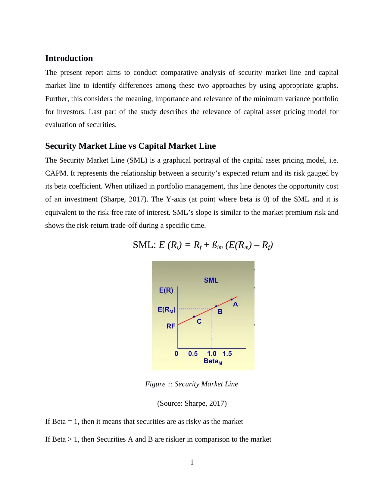
The Security Market Line (SML) is a graphical portrayal of the capital asset pricing model, i.e.
CAPM. It represents the relationship between a security’s expected return and its risk gauged by
its beta coefficient. When utilized in portfolio management, this line denotes the opportunity cost
of an investment (Sharpe, 2017). The Y-axis (at point where beta is 0) of the SML and it is
equivalent to the risk-free rate of interest. SML’s slope is similar to the market premium risk and
shows the risk-return trade-off during a specific time.
SML: E (Ri) = Rf + ßim (E(Rm) – Rf)
Figure 1: Security Market Line
(Source: Sharpe, 2017)
If Beta = 1, then it means that securities are as risky as the market
If Beta > 1, then Securities A and B are riskier in comparison to the market
1
The present report aims to conduct comparative analysis of security market line and capital
market line to identify differences among these two approaches by using appropriate graphs.
Further, this considers the meaning, importance and relevance of the minimum variance portfolio
for investors. Last part of the study describes the relevance of capital asset pricing model for
evaluation of securities.
Security Market Line vs Capital Market Line
The Security Market Line (SML) is a graphical portrayal of the capital asset pricing model, i.e.
CAPM. It represents the relationship between a security’s expected return and its risk gauged by
its beta coefficient. When utilized in portfolio management, this line denotes the opportunity cost
of an investment (Sharpe, 2017). The Y-axis (at point where beta is 0) of the SML and it is
equivalent to the risk-free rate of interest. SML’s slope is similar to the market premium risk and
shows the risk-return trade-off during a specific time.
SML: E (Ri) = Rf + ßim (E(Rm) – Rf)
Figure 1: Security Market Line
(Source: Sharpe, 2017)
If Beta = 1, then it means that securities are as risky as the market
If Beta > 1, then Securities A and B are riskier in comparison to the market
1
Paraphrase This Document
Need a fresh take? Get an instant paraphrase of this document with our AI Paraphraser
If Beta < 1, then Security C is less risky in comparison to the market
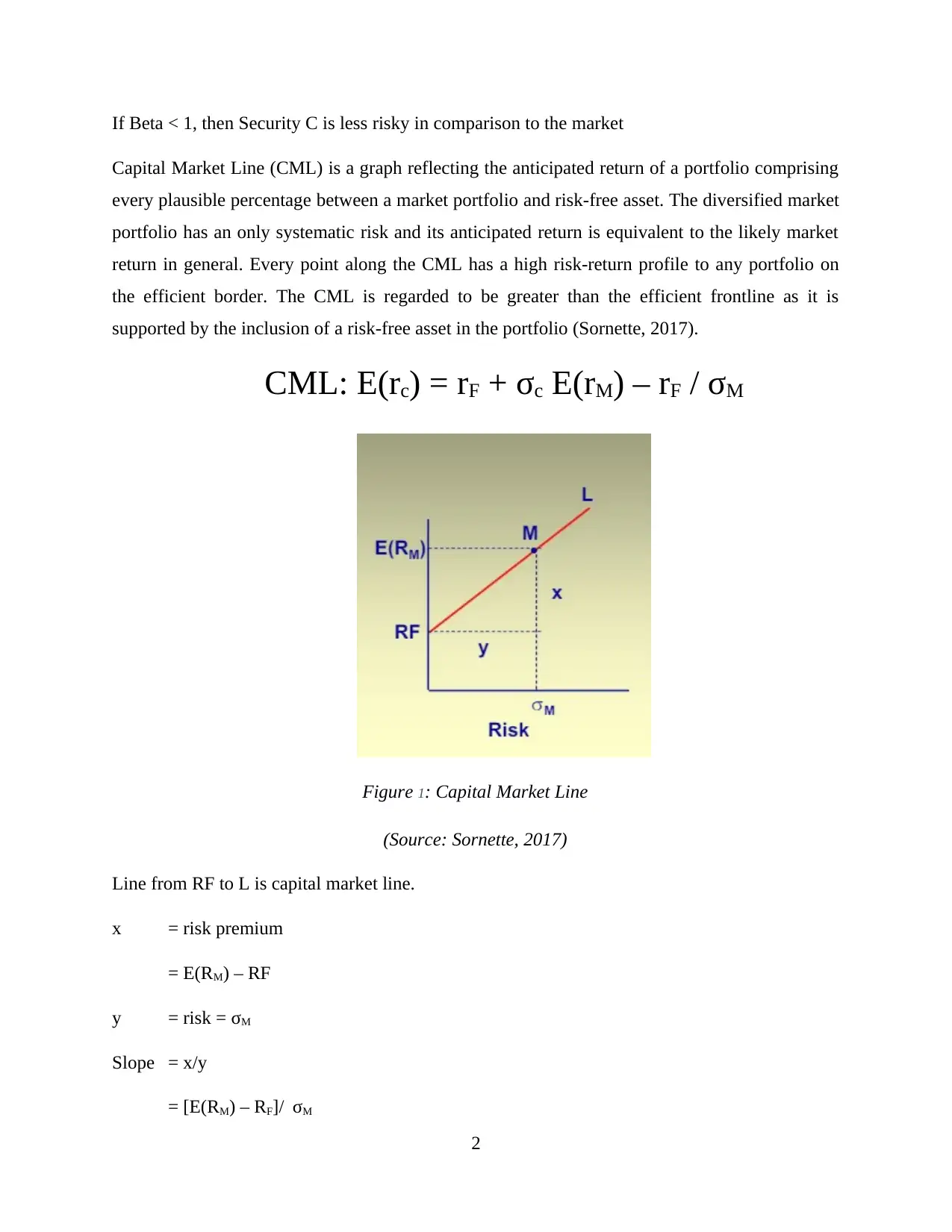
Capital Market Line (CML) is a graph reflecting the anticipated return of a portfolio comprising
every plausible percentage between a market portfolio and risk-free asset. The diversified market
portfolio has an only systematic risk and its anticipated return is equivalent to the likely market
return in general. Every point along the CML has a high risk-return profile to any portfolio on
the efficient border. The CML is regarded to be greater than the efficient frontline as it is
supported by the inclusion of a risk-free asset in the portfolio (Sornette, 2017).
CML: E(rc) = rF + σc E(rM) – rF / σM
Figure 1: Capital Market Line
(Source: Sornette, 2017)
Line from RF to L is capital market line.
x = risk premium
= E(RM) – RF
y = risk = σM
Slope = x/y
= [E(RM) – RF]/ σM
2
y-intercept = RF (Sornette, 2017)
One of the key differences between SML and CML is the manner in which risk elements are
measured. Beta coefficient is the measure of risk elements in the SML. In contrast, standard
deviation determines the risk factors for CML. The SML assesses risk via beta which assists in
identifying of risk contribution by the individual security to the whole portfolio. On the other
hand, assessment of risk in CML is done by means of standard deviation or via a total risk factor
(Hong and Sraer, 2016).
While the SML defines both non-efficiency as well as efficiency of portfolios, while the CML
only shows efficient portfolios. When computing of return, the likely return of the portfolio for
CML is demonstrated alongside the Y-axis. In contrast, the return on securities for SML, is
demonstrated alongside Y axis. For CML, a portfolio’s standard deviation is demonstrated along
the Y-axis. On the other hand, for SML, the Beta of security is demonstrated along the X-axis
(Pilbeam, 2018).
Where the CML determines the risk-free assets and market portfolio, all security elements are
identified by the SML. Unlike the CML, the SML portrays the likely returns of individual assets.
The CML identifies the return or risk for efficient portfolios, and the SML shows the return or
risk for individual shares (Sharpe, 2017). The bottom line is that the CML is regarded to be
better when assessing risk elements.
Importance of Minimum Variance Portfolios
A minimum variance portfolio is a pool of investments with the least volatility, i.e. those
investments which they have less possibility of price variation because they carry the minimum
sensitivity risk. The spread of investments combined together has a lower consequent risk level
relative to the individual risk of every stock. Investors who are not willing to assume big risks
must contemplate taking a minimum variance portfolio (Yang, Couillet and McKay, 2015).
3
⊘ This is a preview!⊘
Do you want full access?
Subscribe today to unlock all pages.
Trusted by 1+ million students worldwide
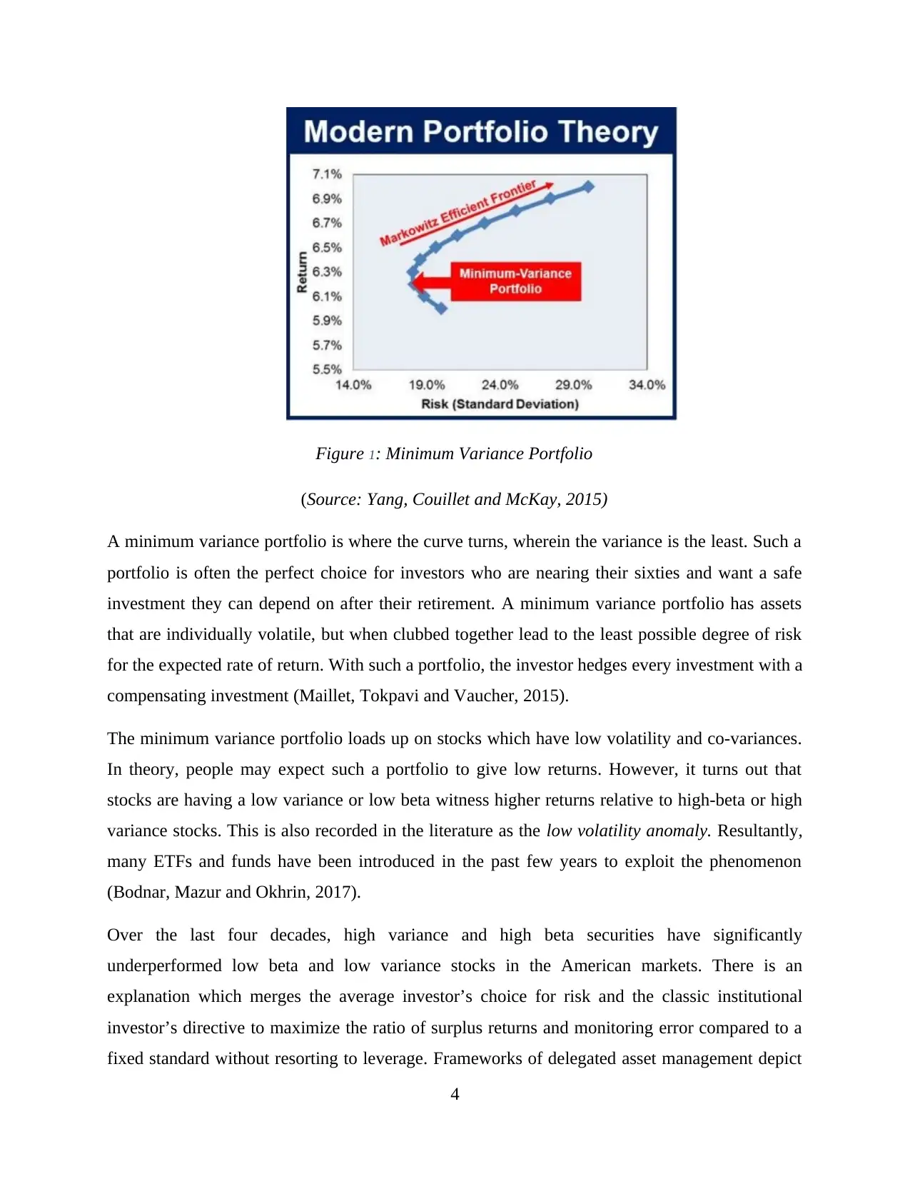
Figure 1: Minimum Variance Portfolio
(Source: Yang, Couillet and McKay, 2015)
A minimum variance portfolio is where the curve turns, wherein the variance is the least. Such a
portfolio is often the perfect choice for investors who are nearing their sixties and want a safe
investment they can depend on after their retirement. A minimum variance portfolio has assets
that are individually volatile, but when clubbed together lead to the least possible degree of risk
for the expected rate of return. With such a portfolio, the investor hedges every investment with a
compensating investment (Maillet, Tokpavi and Vaucher, 2015).
The minimum variance portfolio loads up on stocks which have low volatility and co-variances.
In theory, people may expect such a portfolio to give low returns. However, it turns out that
stocks are having a low variance or low beta witness higher returns relative to high-beta or high
variance stocks. This is also recorded in the literature as the low volatility anomaly. Resultantly,
many ETFs and funds have been introduced in the past few years to exploit the phenomenon
(Bodnar, Mazur and Okhrin, 2017).
Over the last four decades, high variance and high beta securities have significantly
underperformed low beta and low variance stocks in the American markets. There is an
explanation which merges the average investor’s choice for risk and the classic institutional
investor’s directive to maximize the ratio of surplus returns and monitoring error compared to a
fixed standard without resorting to leverage. Frameworks of delegated asset management depict
4
Paraphrase This Document
Need a fresh take? Get an instant paraphrase of this document with our AI Paraphraser
that these directives dissuade arbitrage in both low beta - high alpha, and high beta - low alpha
securities (Kempf and Memmel, 2006). This reasoning is in alignment with many facets of the
low variance anomaly entailing why it has fostered in the past few years even as the dominance
of institutional investors has increased.
Minimum market portfolios are more flexible in market downturns. As the business cycle finally
recoups, a minimum variance portfolio tends to ensure compounding performance in comparison
to return provided by market. One of the biggest advantages of the minimum variance portfolio
is that it really eliminates expected returns from the optimization which are tough to handle. As
the minimum variance portfolios have the sole goal of decreasing risk, instead of striving to
optimize the reward-risk ratio. Further, minimum variance portfolio optimization results in
noticeable attention on low variance securities in against of the cost of exploiting correlation
properties (Clarke, De Silva and Thorley, 2011). While MVP is not ideal portfolios, but they
might be appropriate for investors who intend to load up on low-risk stocks. As estimation risk
natural to projected returns is a known aspect, the fact that the MVP depends just on risk criteria
is an attractive attribute.
The relevance of the CAPM equation
The Capital Asset Pricing Model (CAPM) is a framework which computes the expected return
on the basis of the projected rate of return on the market, the beta coefficient of the security and
risk-free rate. The equation for CAPM to calculate the rate of return is
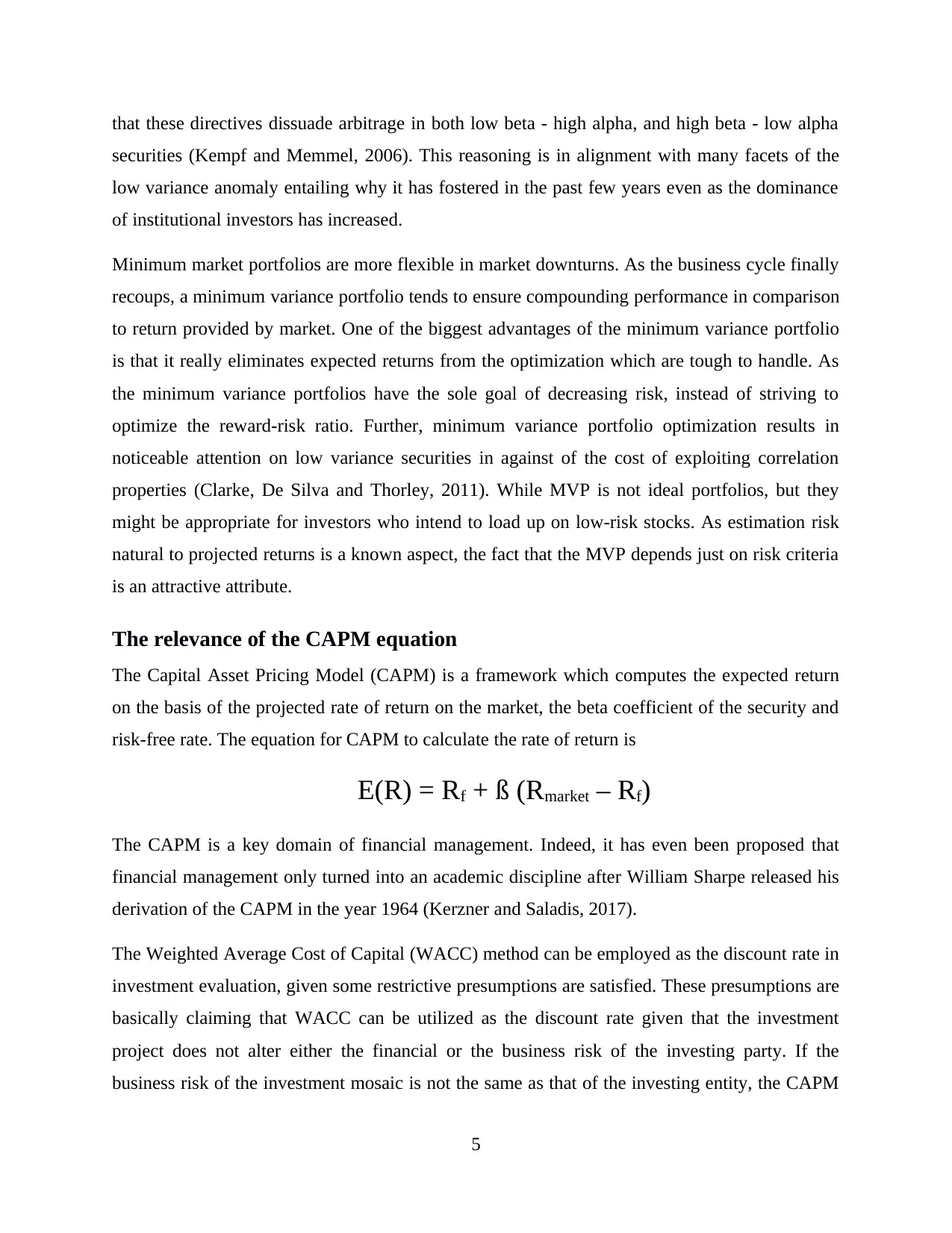
E(R) = Rf + ß (Rmarket – Rf)
The CAPM is a key domain of financial management. Indeed, it has even been proposed that
financial management only turned into an academic discipline after William Sharpe released his
derivation of the CAPM in the year 1964 (Kerzner and Saladis, 2017).
The Weighted Average Cost of Capital (WACC) method can be employed as the discount rate in
investment evaluation, given some restrictive presumptions are satisfied. These presumptions are
basically claiming that WACC can be utilized as the discount rate given that the investment
project does not alter either the financial or the business risk of the investing party. If the
business risk of the investment mosaic is not the same as that of the investing entity, the CAPM
5
securities (Kempf and Memmel, 2006). This reasoning is in alignment with many facets of the
low variance anomaly entailing why it has fostered in the past few years even as the dominance
of institutional investors has increased.
Minimum market portfolios are more flexible in market downturns. As the business cycle finally
recoups, a minimum variance portfolio tends to ensure compounding performance in comparison
to return provided by market. One of the biggest advantages of the minimum variance portfolio
is that it really eliminates expected returns from the optimization which are tough to handle. As
the minimum variance portfolios have the sole goal of decreasing risk, instead of striving to
optimize the reward-risk ratio. Further, minimum variance portfolio optimization results in
noticeable attention on low variance securities in against of the cost of exploiting correlation
properties (Clarke, De Silva and Thorley, 2011). While MVP is not ideal portfolios, but they
might be appropriate for investors who intend to load up on low-risk stocks. As estimation risk
natural to projected returns is a known aspect, the fact that the MVP depends just on risk criteria
is an attractive attribute.
The relevance of the CAPM equation
The Capital Asset Pricing Model (CAPM) is a framework which computes the expected return
on the basis of the projected rate of return on the market, the beta coefficient of the security and
risk-free rate. The equation for CAPM to calculate the rate of return is
E(R) = Rf + ß (Rmarket – Rf)
The CAPM is a key domain of financial management. Indeed, it has even been proposed that
financial management only turned into an academic discipline after William Sharpe released his
derivation of the CAPM in the year 1964 (Kerzner and Saladis, 2017).
The Weighted Average Cost of Capital (WACC) method can be employed as the discount rate in
investment evaluation, given some restrictive presumptions are satisfied. These presumptions are
basically claiming that WACC can be utilized as the discount rate given that the investment
project does not alter either the financial or the business risk of the investing party. If the
business risk of the investment mosaic is not the same as that of the investing entity, the CAPM
5
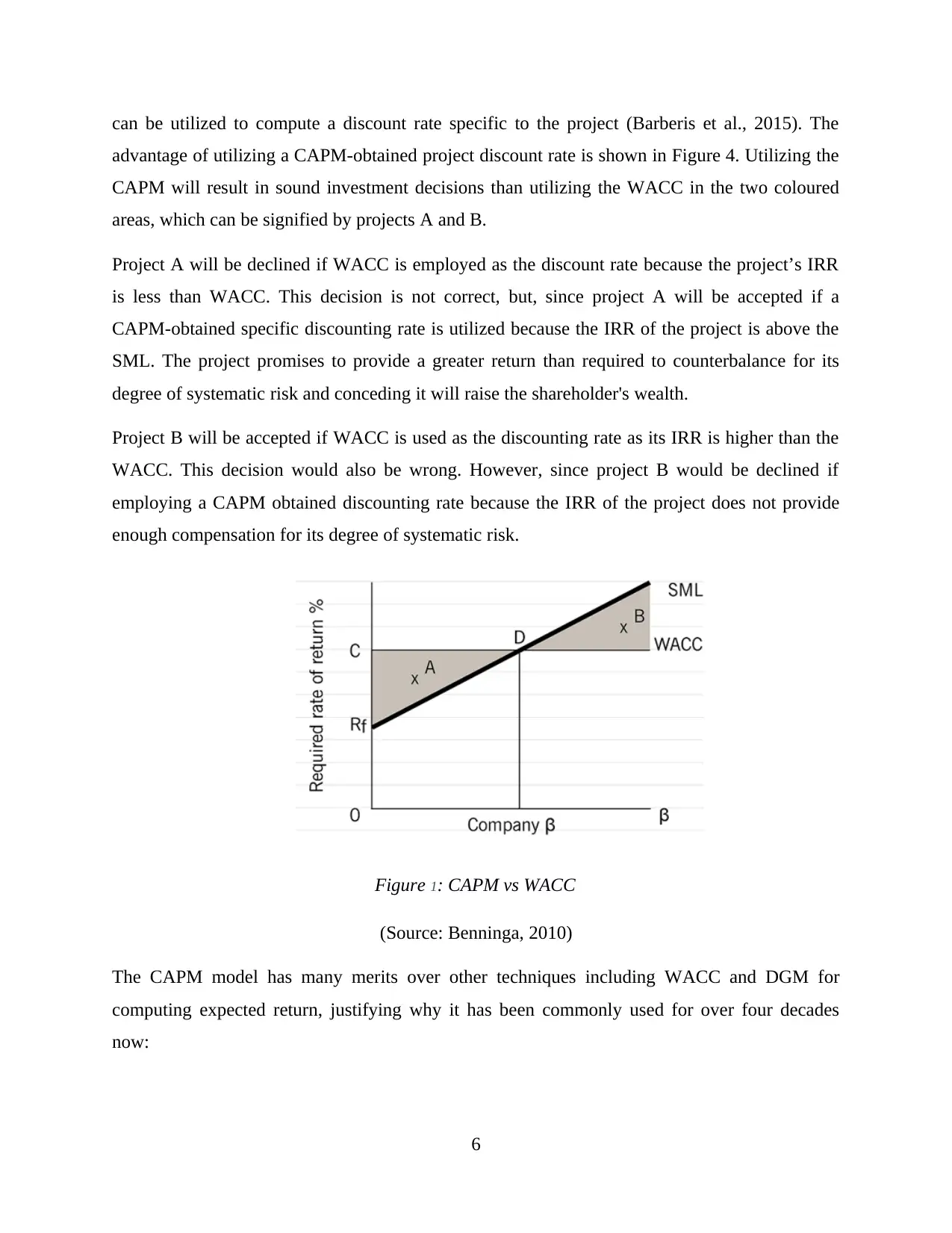
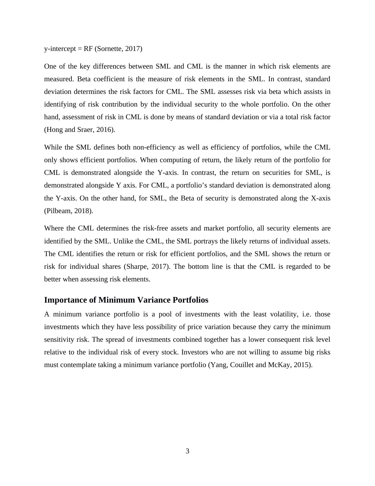
can be utilized to compute a discount rate specific to the project (Barberis et al., 2015). The
advantage of utilizing a CAPM-obtained project discount rate is shown in Figure 4. Utilizing the
CAPM will result in sound investment decisions than utilizing the WACC in the two coloured
areas, which can be signified by projects A and B.
Project A will be declined if WACC is employed as the discount rate because the project’s IRR
is less than WACC. This decision is not correct, but, since project A will be accepted if a
CAPM-obtained specific discounting rate is utilized because the IRR of the project is above the
SML. The project promises to provide a greater return than required to counterbalance for its
degree of systematic risk and conceding it will raise the shareholder's wealth.
Project B will be accepted if WACC is used as the discounting rate as its IRR is higher than the
WACC. This decision would also be wrong. However, since project B would be declined if
employing a CAPM obtained discounting rate because the IRR of the project does not provide
enough compensation for its degree of systematic risk.
Figure 1: CAPM vs WACC
(Source: Benninga, 2010)
The CAPM model has many merits over other techniques including WACC and DGM for
computing expected return, justifying why it has been commonly used for over four decades
now:
6
⊘ This is a preview!⊘
Do you want full access?
Subscribe today to unlock all pages.
Trusted by 1+ million students worldwide
It only considers systematic risk, showing a real scenario in which majority investors
have a diverse portfolio supported by elimination of unsystematic risk in an essential
manner.
It is a theoretically obtained relationship among expected return and systematic risk. This
approach is prone to regular empirical testing and research (Kerzner and Saladis, 2017).
It is often viewed as a much advanced and better technique to calculate the cost of equity
in comparison to the Dividend Growth Model (DGM) in that it clearly considers a firm’s
degree of systematic risk compared to the share market as a whole.
It is evidently better than WACC in offering discount rates for utilization in investment
evaluation.
When businesses examine prospects, if the business combination and financing vary from
the existing business, then other expected return computations like WACC are rendered
useless. However, CAPM can be used in this situation (Bekaert and Hodrick, 2017).
The bottom line is that no model is ideal. However, each must have some attributes
which render it helpful and suitable. CAPM, though criticized for some of its unrealistic
presumptions, offers a more usable result than either WACC or DDM in many scenarios. It is
stress-tested and easily computed, and when employed together with other elements of an
investment mosaic, it can offer unmatched yield data which can remove or support a likely
investment (Petty et al., 2015).
Conclusion
By considering the present study conclusion can be drawn that SML and CML both assist in
evaluating efficiency on portfolios but on the basis of different backgrounds. By the application
of the minimum variance portfolio, an investor can attain expected returns from the optimization
which are tough to handle. Further, CAPM is viable in comparison to other equations as it covers
overall aspects concerned with the market for analysis of securities.
7
Paraphrase This Document
Need a fresh take? Get an instant paraphrase of this document with our AI Paraphraser
References
Barberis, N., Greenwood, R., Jin, L. and Shleifer, A., 2015. X-CAPM: An extrapolative capital
asset pricing model. Journal of financial economics, 115(1), pp.1-24.
Bekaert, G. and Hodrick, R., 2017. International financial management. Cambridge University
Press.
Benninga, S., 2010. Principles of finance with excel. OUP Catalogue.
Bodnar, T., Mazur, S. and Okhrin, Y., 2017. Bayesian estimation of the global minimum
variance portfolio. European Journal of Operational Research, 256(1), pp.292-307.
Clarke, R., De Silva, H. and Thorley, S., 2011. Minimum-variance portfolio
composition. Journal of Portfolio Management, 37(2), p.31.
Hong, H. and Sraer, D.A., 2016. Speculative betas. The Journal of Finance, 71(5), pp.2095-
2144.
Kempf, A. and Memmel, C., 2006. Estimating the global minimum variance
portfolio. Schmalenbach Business Review, 58(4), pp.332-348.
Kerzner, H. and Saladis, F.P., 2017. Project management workbook and PMP/CAPM exam
study guide. John Wiley & Sons.
Maillet, B., Tokpavi, S. and Vaucher, B., 2015. Global minimum variance portfolio optimisation
under some model risk: A robust regression-based approach. European Journal of Operational
Research, 244(1), pp.289-299.
Petty, J.W., Titman, S., Keown, A.J., Martin, P., Martin, J.D. and Burrow, M., 2015. Financial
management: Principles and applications. Pearson Higher Education AU.
Pilbeam, K., 2018. Finance & financial markets. Macmillan International Higher Education.
Sharpe, W., 2017. Capital Market Theory, Efficiency, and Imperfections. Quantitative Financial
Analytics: The Path to Investment Profits, p.445.
Sornette, D., 2017. Why stock markets crash: critical events in complex financial systems.
Princeton University Press.
Yang, L., Couillet, R. and McKay, M.R., 2015. A robust statistics approach to minimum
variance portfolio optimization. IEEE Transactions on Signal Processing, 63(24), pp.6684-6697.
8
1 out of 11
Related Documents


Your All-in-One AI-Powered Toolkit for Academic Success.
+13062052269
info@desklib.com
Available 24*7 on WhatsApp / Email
![[object Object]](/_next/static/media/star-bottom.7253800d.svg)
Unlock your academic potential
Copyright © 2020–2026 A2Z Services. All Rights Reserved. Developed and managed by ZUCOL.