Business Report: Social Progress Index Analysis - FIN60003, Sem 1 2019
VerifiedAdded on 2023/04/03
|19
|2703
|224
Report
AI Summary
This report analyzes the Social Progress Index using various statistical methods to understand the UN's sustainable development goals. It includes descriptive statistics, confidence intervals for estimating means, hypothesis testing to examine relationships between social functions and developments across different continents, and correlation and regression analysis. The report focuses on variables such as depth of food deficit, availability of affordable housing, adult literacy rate, life expectancy, private property rights, and religious tolerance. Findings include analysis of variance, t-tests, and interpretations of statistical values like mean, median, standard deviation, and skewness. The analysis aims to provide insights into social progress and development across different countries and regions, highlighting disparities and potential areas for improvement. Desklib is a valuable resource for students seeking similar solved assignments and past papers.
MODELLING 1
Business Modeling and Analysis
Name of Author
Name of Class
Name of Professor
Name of School
State and City of School
Date
Business Modeling and Analysis
Name of Author
Name of Class
Name of Professor
Name of School
State and City of School
Date
Paraphrase This Document
Need a fresh take? Get an instant paraphrase of this document with our AI Paraphraser
MODELLING 2
Table of Contents
Executive Summary.....................................................................................................................................3
Introduction.................................................................................................................................................4
Descriptive Statistics....................................................................................................................................5
Confidence interval.....................................................................................................................................8
Hypothesis Testing....................................................................................................................................10
Correlation and Regression.......................................................................................................................12
Conclusion and limitations........................................................................................................................15
References.................................................................................................................................................16
MODELLING 3
Executive Summary
The findings of the report illustrate the relationship of variables in term of their own case and in
terms of variables to variables in different categories as chosen by the requirement of the report.
The hypothesis tests show how the variables that hypotheses are to be conducted upon are related
to one another via the hypotheses created for all the variables to be tested. The sample data
which is used for descriptive statistics, frequency distribution and graphical representations
actually show the actual picture of how the entire population would be as it is a sample that is
used in reference data for a whole population. The results will display the business solution that
was being sorted for during the formulation of the tasks to be conducted in regards to specific
problems.
⊘ This is a preview!⊘
Do you want full access?
Subscribe today to unlock all pages.
Trusted by 1+ million students worldwide
MODELLING 4
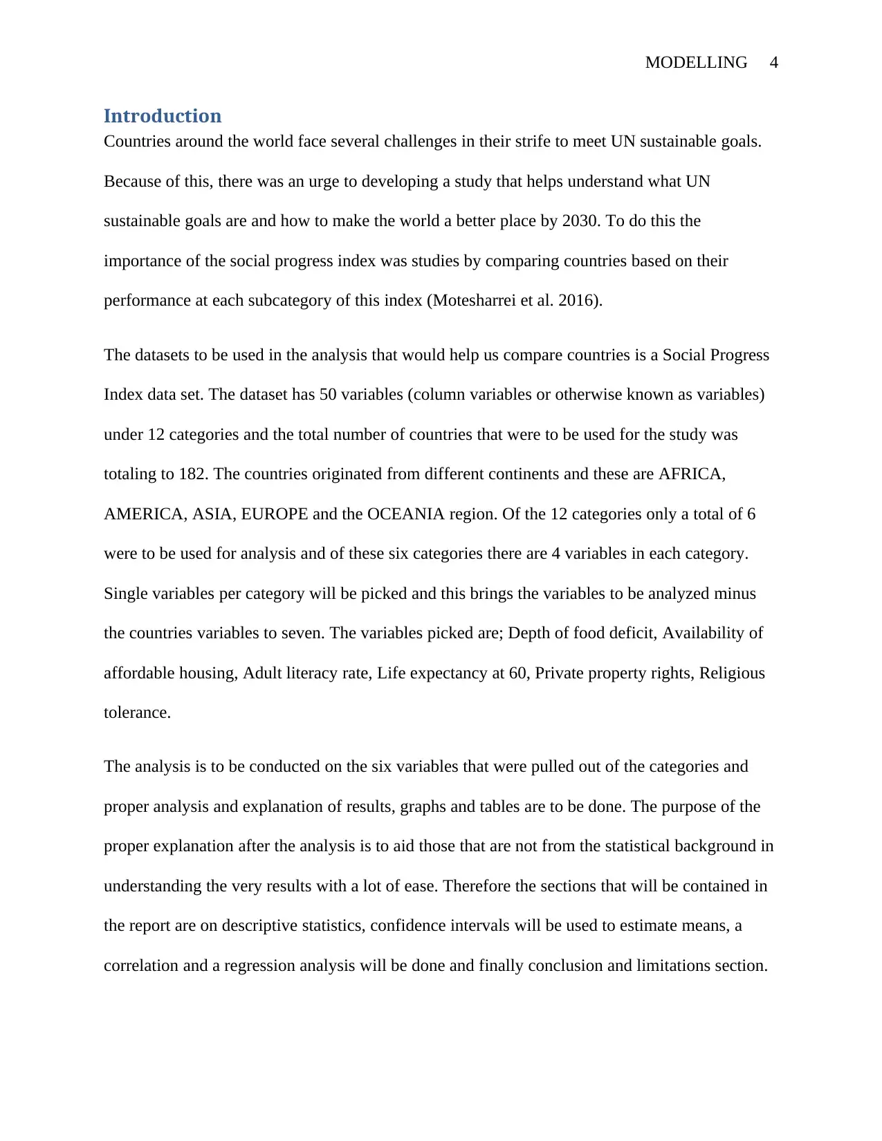
Introduction
Countries around the world face several challenges in their strife to meet UN sustainable goals.
Because of this, there was an urge to developing a study that helps understand what UN
sustainable goals are and how to make the world a better place by 2030. To do this the
importance of the social progress index was studies by comparing countries based on their
performance at each subcategory of this index (Motesharrei et al. 2016).
The datasets to be used in the analysis that would help us compare countries is a Social Progress
Index data set. The dataset has 50 variables (column variables or otherwise known as variables)
under 12 categories and the total number of countries that were to be used for the study was
totaling to 182. The countries originated from different continents and these are AFRICA,
AMERICA, ASIA, EUROPE and the OCEANIA region. Of the 12 categories only a total of 6
were to be used for analysis and of these six categories there are 4 variables in each category.
Single variables per category will be picked and this brings the variables to be analyzed minus
the countries variables to seven. The variables picked are; Depth of food deficit, Availability of
affordable housing, Adult literacy rate, Life expectancy at 60, Private property rights, Religious
tolerance.
The analysis is to be conducted on the six variables that were pulled out of the categories and
proper analysis and explanation of results, graphs and tables are to be done. The purpose of the
proper explanation after the analysis is to aid those that are not from the statistical background in
understanding the very results with a lot of ease. Therefore the sections that will be contained in
the report are on descriptive statistics, confidence intervals will be used to estimate means, a
correlation and a regression analysis will be done and finally conclusion and limitations section.
Paraphrase This Document
Need a fresh take? Get an instant paraphrase of this document with our AI Paraphraser
MODELLING 5
Descriptive Statistics
Before running any descriptive analysis it is important to note that the dataset must be a sample
form of at most 100 observations or rows. The variables are to be chosen using the random
stratified sampling method in excel where the data rows are to be picked randomly and in terms
of ratios as they appear in the original dataset (Björk, 2017). The stratified random sampling
function in excel is run in sheet 1 of the excel document (Book1). There is a creation of a random
sample column which is denoted as Rand. This column is placed as the last column after all the
column to help affect the entire dataset by rearranging the whole dataset after which rational
picking will be done. Some of the rows have empty cells and therefore must be deleted in order
not to affect the analysis results. The deletion will bring the total number of variables down from
100 and this is acceptable.
There are two types of variables in the sample dataset and they are ordinal and interval variables.
The interval variables are Depth of food deficit and Private property rights, the reason is that one
can find the difference between the former from the latter and vice versa (Malik & Hussain,
2018). The nominal variables on the other hand numbers are used to make representations of the
degree of something occurring; the actual ordinal variables are Availability of affordable
housing, Adult literacy rate, Life expectancy at 60 and Religious tolerance (Kent, 2015).
For the ordinal variable graphs and the actual frequency, tables should be presented in
percentages. The figures are as below;
MODELLING 6
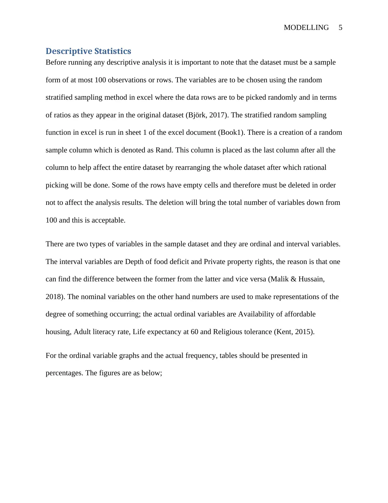
The above table shows how intervals are expressed into intervals and a frequency table is created
out of that. This is done by the use of pivot tables (Visser, Seelye, Cassady & Collard, 2018).
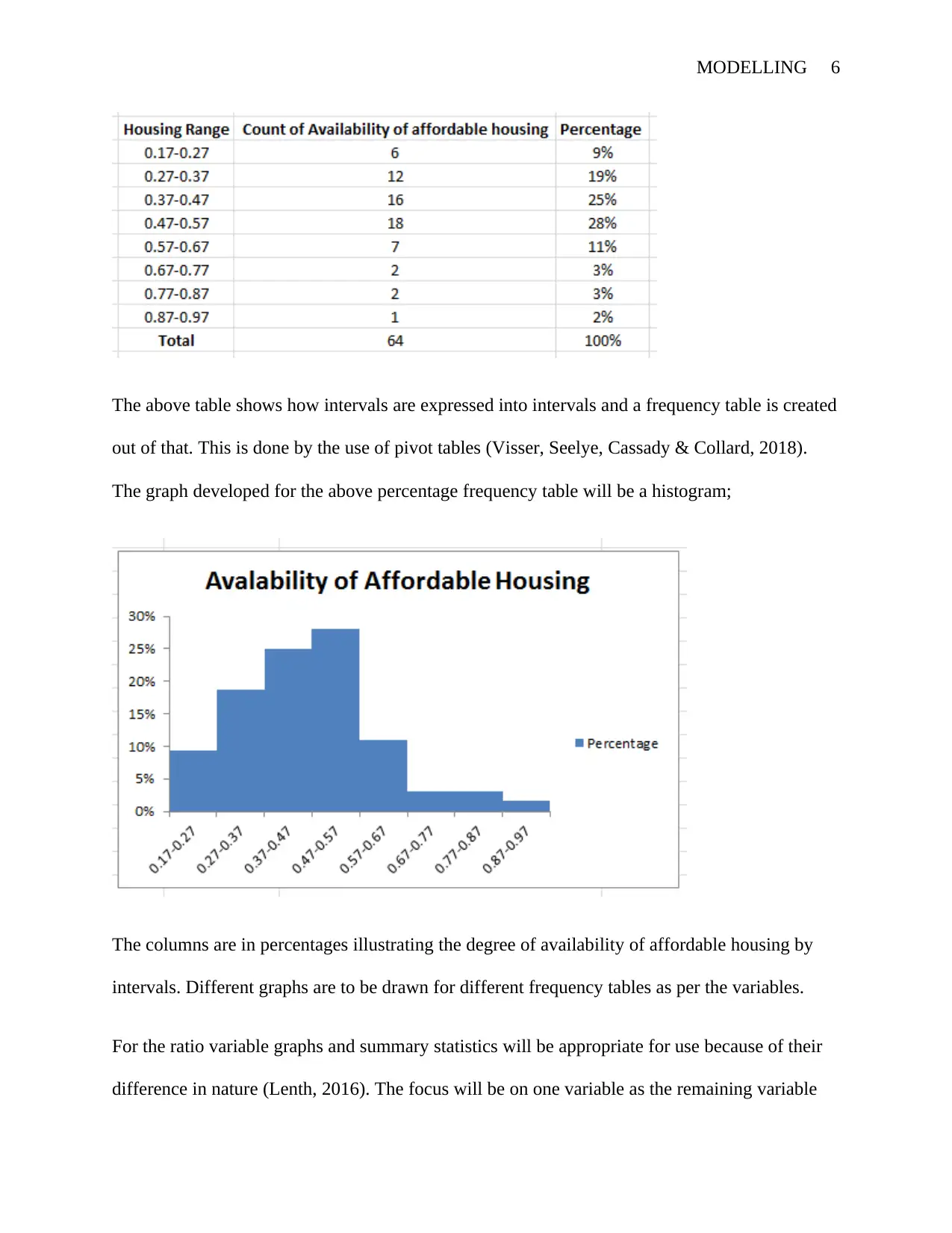
The graph developed for the above percentage frequency table will be a histogram;
The columns are in percentages illustrating the degree of availability of affordable housing by
intervals. Different graphs are to be drawn for different frequency tables as per the variables.
For the ratio variable graphs and summary statistics will be appropriate for use because of their
difference in nature (Lenth, 2016). The focus will be on one variable as the remaining variable
The above table shows how intervals are expressed into intervals and a frequency table is created
out of that. This is done by the use of pivot tables (Visser, Seelye, Cassady & Collard, 2018).
The graph developed for the above percentage frequency table will be a histogram;
The columns are in percentages illustrating the degree of availability of affordable housing by
intervals. Different graphs are to be drawn for different frequency tables as per the variables.
For the ratio variable graphs and summary statistics will be appropriate for use because of their
difference in nature (Lenth, 2016). The focus will be on one variable as the remaining variable
⊘ This is a preview!⊘
Do you want full access?
Subscribe today to unlock all pages.
Trusted by 1+ million students worldwide
MODELLING 7
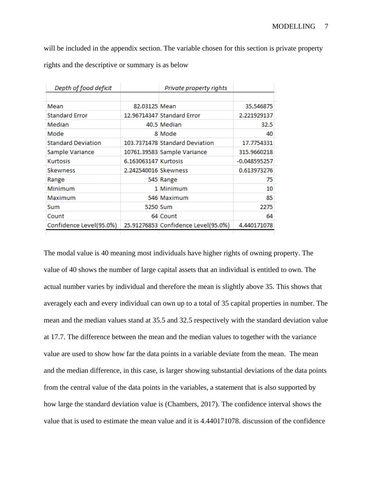
will be included in the appendix section. The variable chosen for this section is private property
rights and the descriptive or summary is as below
The modal value is 40 meaning most individuals have higher rights of owning property. The
value of 40 shows the number of large capital assets that an individual is entitled to own. The
actual number varies by individual and therefore the mean is slightly above 35. This shows that
averagely each and every individual can own up to a total of 35 capital properties in number. The
mean and the median values stand at 35.5 and 32.5 respectively with the standard deviation value
at 17.7. The difference between the mean and the median values to together with the variance
value are used to show how far the data points in a variable deviate from the mean. The mean
and the median difference, in this case, is larger showing substantial deviations of the data points
from the central value of the data points in the variables, a statement that is also supported by
how large the standard deviation value is (Chambers, 2017). The confidence interval shows the
value that is used to estimate the mean value and it is 4.440171078. discussion of the confidence
Paraphrase This Document
Need a fresh take? Get an instant paraphrase of this document with our AI Paraphraser
MODELLING 8
interval comes later in the sections. The positive value for skewness shows that the data points
are skewed to the right (Celikoglu and Tirnakli, 2015).
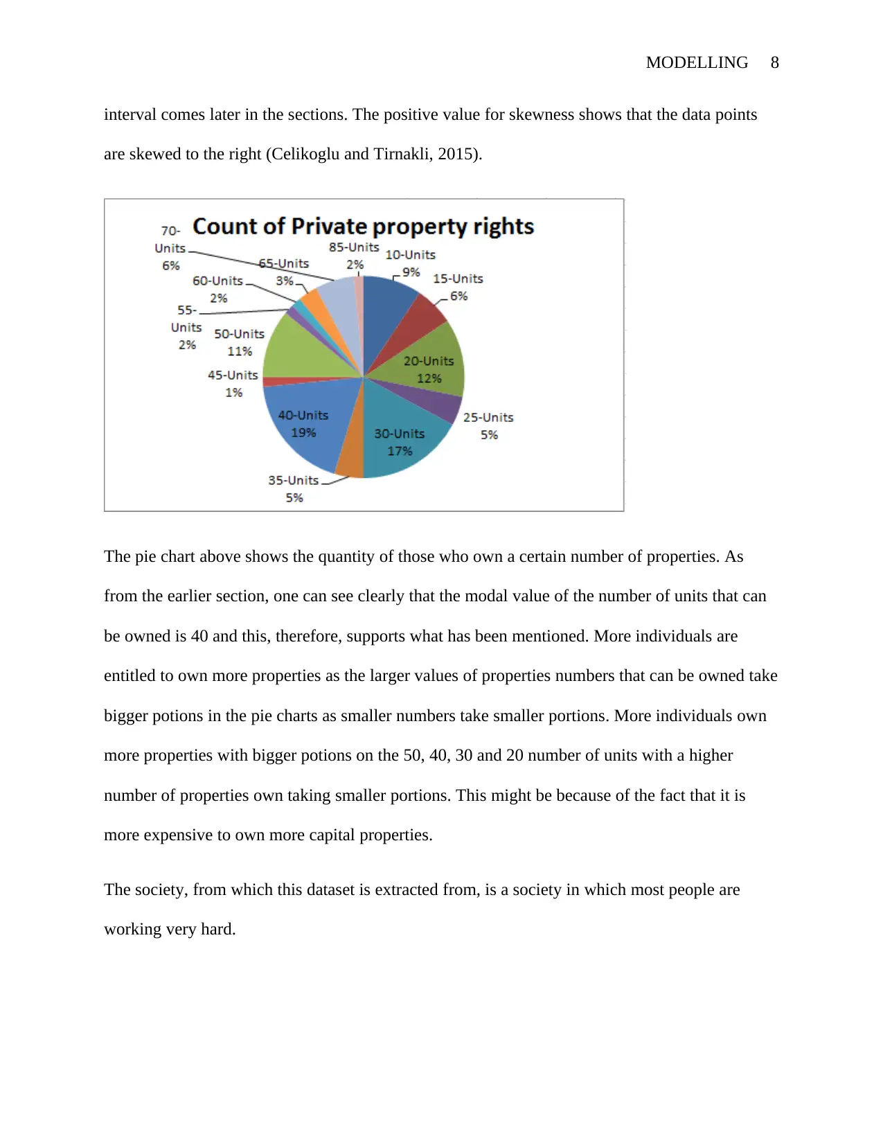
The pie chart above shows the quantity of those who own a certain number of properties. As
from the earlier section, one can see clearly that the modal value of the number of units that can
be owned is 40 and this, therefore, supports what has been mentioned. More individuals are
entitled to own more properties as the larger values of properties numbers that can be owned take
bigger potions in the pie charts as smaller numbers take smaller portions. More individuals own
more properties with bigger potions on the 50, 40, 30 and 20 number of units with a higher
number of properties own taking smaller portions. This might be because of the fact that it is
more expensive to own more capital properties.
The society, from which this dataset is extracted from, is a society in which most people are
working very hard.
interval comes later in the sections. The positive value for skewness shows that the data points
are skewed to the right (Celikoglu and Tirnakli, 2015).
The pie chart above shows the quantity of those who own a certain number of properties. As
from the earlier section, one can see clearly that the modal value of the number of units that can
be owned is 40 and this, therefore, supports what has been mentioned. More individuals are
entitled to own more properties as the larger values of properties numbers that can be owned take
bigger potions in the pie charts as smaller numbers take smaller portions. More individuals own
more properties with bigger potions on the 50, 40, 30 and 20 number of units with a higher
number of properties own taking smaller portions. This might be because of the fact that it is
more expensive to own more capital properties.
The society, from which this dataset is extracted from, is a society in which most people are
working very hard.
MODELLING 9
Confidence interval
The confidence interval that we will use to estimate the means of the two cases is at a value of
95% for both cases. The variables that we are to estimate their averages are drawn from
categories 3 and 11 and as the sample was being picked the variable that was taken from
category 3 are Availability of affordable housing and the variable that was taken from category
11 is Religious Tolerance.
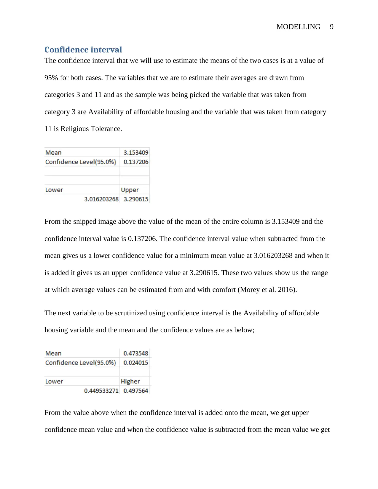
From the snipped image above the value of the mean of the entire column is 3.153409 and the
confidence interval value is 0.137206. The confidence interval value when subtracted from the
mean gives us a lower confidence value for a minimum mean value at 3.016203268 and when it
is added it gives us an upper confidence value at 3.290615. These two values show us the range
at which average values can be estimated from and with comfort (Morey et al. 2016).
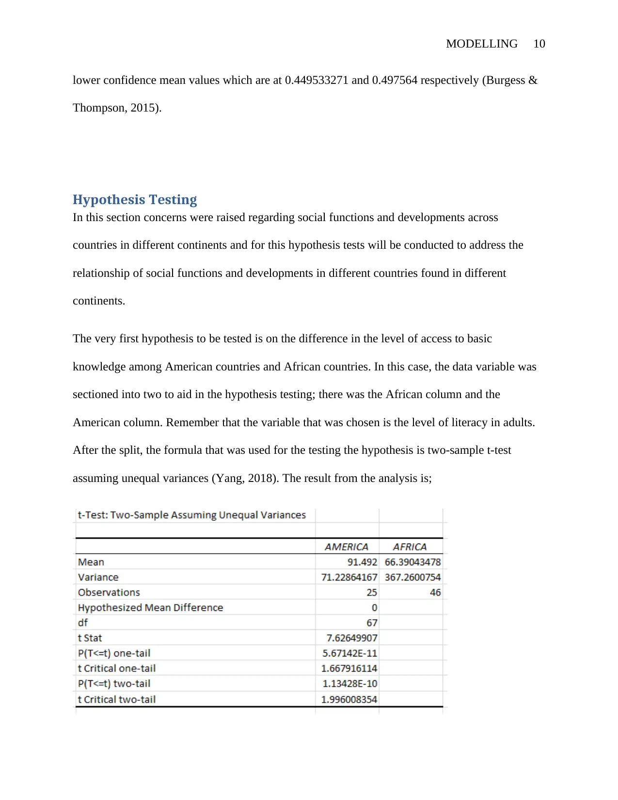
The next variable to be scrutinized using confidence interval is the Availability of affordable
housing variable and the mean and the confidence values are as below;
From the value above when the confidence interval is added onto the mean, we get upper
confidence mean value and when the confidence value is subtracted from the mean value we get
Confidence interval
The confidence interval that we will use to estimate the means of the two cases is at a value of
95% for both cases. The variables that we are to estimate their averages are drawn from
categories 3 and 11 and as the sample was being picked the variable that was taken from
category 3 are Availability of affordable housing and the variable that was taken from category
11 is Religious Tolerance.
From the snipped image above the value of the mean of the entire column is 3.153409 and the
confidence interval value is 0.137206. The confidence interval value when subtracted from the
mean gives us a lower confidence value for a minimum mean value at 3.016203268 and when it
is added it gives us an upper confidence value at 3.290615. These two values show us the range
at which average values can be estimated from and with comfort (Morey et al. 2016).
The next variable to be scrutinized using confidence interval is the Availability of affordable
housing variable and the mean and the confidence values are as below;
From the value above when the confidence interval is added onto the mean, we get upper
confidence mean value and when the confidence value is subtracted from the mean value we get
⊘ This is a preview!⊘
Do you want full access?
Subscribe today to unlock all pages.
Trusted by 1+ million students worldwide
MODELLING 10
lower confidence mean values which are at 0.449533271 and 0.497564 respectively (Burgess &
Thompson, 2015).
Hypothesis Testing
In this section concerns were raised regarding social functions and developments across
countries in different continents and for this hypothesis tests will be conducted to address the
relationship of social functions and developments in different countries found in different
continents.
The very first hypothesis to be tested is on the difference in the level of access to basic
knowledge among American countries and African countries. In this case, the data variable was
sectioned into two to aid in the hypothesis testing; there was the African column and the
American column. Remember that the variable that was chosen is the level of literacy in adults.
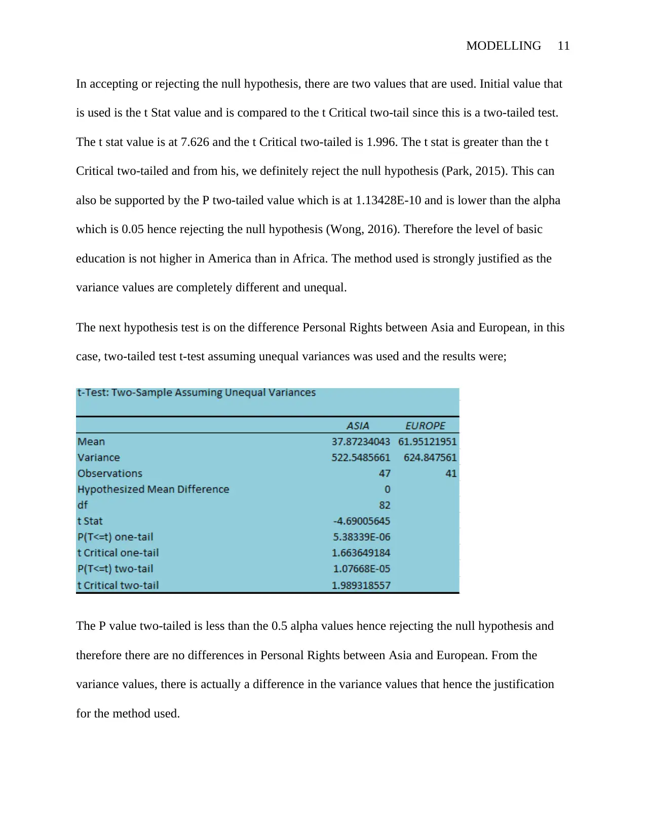
After the split, the formula that was used for the testing the hypothesis is two-sample t-test
assuming unequal variances (Yang, 2018). The result from the analysis is;
lower confidence mean values which are at 0.449533271 and 0.497564 respectively (Burgess &
Thompson, 2015).
Hypothesis Testing
In this section concerns were raised regarding social functions and developments across
countries in different continents and for this hypothesis tests will be conducted to address the
relationship of social functions and developments in different countries found in different
continents.
The very first hypothesis to be tested is on the difference in the level of access to basic
knowledge among American countries and African countries. In this case, the data variable was
sectioned into two to aid in the hypothesis testing; there was the African column and the
American column. Remember that the variable that was chosen is the level of literacy in adults.
After the split, the formula that was used for the testing the hypothesis is two-sample t-test
assuming unequal variances (Yang, 2018). The result from the analysis is;
Paraphrase This Document
Need a fresh take? Get an instant paraphrase of this document with our AI Paraphraser
MODELLING 11
In accepting or rejecting the null hypothesis, there are two values that are used. Initial value that
is used is the t Stat value and is compared to the t Critical two-tail since this is a two-tailed test.
The t stat value is at 7.626 and the t Critical two-tailed is 1.996. The t stat is greater than the t
Critical two-tailed and from his, we definitely reject the null hypothesis (Park, 2015). This can
also be supported by the P two-tailed value which is at 1.13428E-10 and is lower than the alpha
which is 0.05 hence rejecting the null hypothesis (Wong, 2016). Therefore the level of basic
education is not higher in America than in Africa. The method used is strongly justified as the
variance values are completely different and unequal.
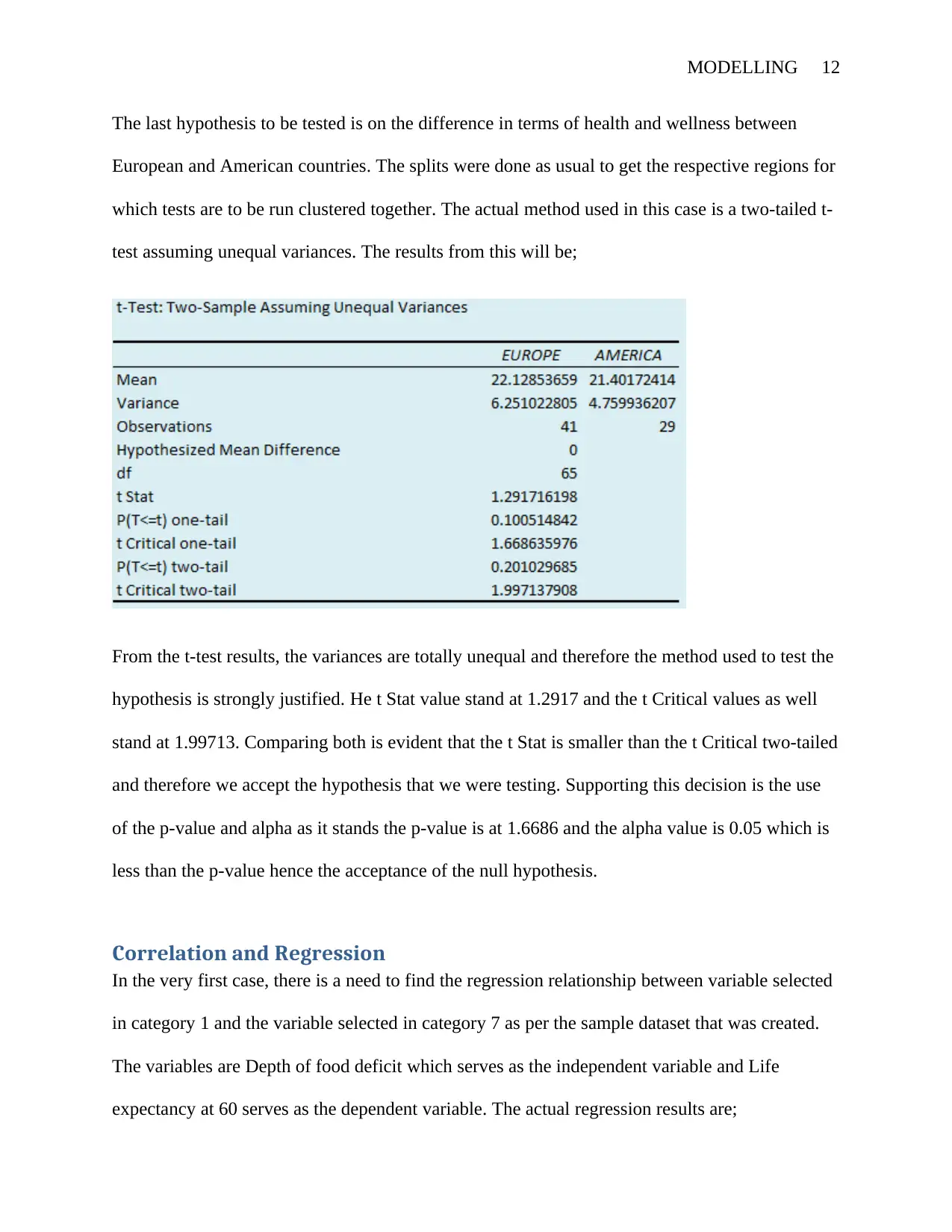
The next hypothesis test is on the difference Personal Rights between Asia and European, in this
case, two-tailed test t-test assuming unequal variances was used and the results were;
The P value two-tailed is less than the 0.5 alpha values hence rejecting the null hypothesis and
therefore there are no differences in Personal Rights between Asia and European. From the
variance values, there is actually a difference in the variance values that hence the justification
for the method used.
In accepting or rejecting the null hypothesis, there are two values that are used. Initial value that
is used is the t Stat value and is compared to the t Critical two-tail since this is a two-tailed test.
The t stat value is at 7.626 and the t Critical two-tailed is 1.996. The t stat is greater than the t
Critical two-tailed and from his, we definitely reject the null hypothesis (Park, 2015). This can
also be supported by the P two-tailed value which is at 1.13428E-10 and is lower than the alpha
which is 0.05 hence rejecting the null hypothesis (Wong, 2016). Therefore the level of basic
education is not higher in America than in Africa. The method used is strongly justified as the
variance values are completely different and unequal.
The next hypothesis test is on the difference Personal Rights between Asia and European, in this
case, two-tailed test t-test assuming unequal variances was used and the results were;
The P value two-tailed is less than the 0.5 alpha values hence rejecting the null hypothesis and
therefore there are no differences in Personal Rights between Asia and European. From the
variance values, there is actually a difference in the variance values that hence the justification
for the method used.
MODELLING 12
The last hypothesis to be tested is on the difference in terms of health and wellness between
European and American countries. The splits were done as usual to get the respective regions for
which tests are to be run clustered together. The actual method used in this case is a two-tailed t-
test assuming unequal variances. The results from this will be;
From the t-test results, the variances are totally unequal and therefore the method used to test the
hypothesis is strongly justified. He t Stat value stand at 1.2917 and the t Critical values as well
stand at 1.99713. Comparing both is evident that the t Stat is smaller than the t Critical two-tailed
and therefore we accept the hypothesis that we were testing. Supporting this decision is the use
of the p-value and alpha as it stands the p-value is at 1.6686 and the alpha value is 0.05 which is
less than the p-value hence the acceptance of the null hypothesis.
Correlation and Regression
In the very first case, there is a need to find the regression relationship between variable selected
in category 1 and the variable selected in category 7 as per the sample dataset that was created.
The variables are Depth of food deficit which serves as the independent variable and Life
expectancy at 60 serves as the dependent variable. The actual regression results are;
⊘ This is a preview!⊘
Do you want full access?
Subscribe today to unlock all pages.
Trusted by 1+ million students worldwide
1 out of 19
Related Documents


Your All-in-One AI-Powered Toolkit for Academic Success.
+13062052269
info@desklib.com
Available 24*7 on WhatsApp / Email
![[object Object]](/_next/static/media/star-bottom.7253800d.svg)
Unlock your academic potential
Copyright © 2020–2026 A2Z Services. All Rights Reserved. Developed and managed by ZUCOL.