ACC544, Decision Support Tools: Finance Assignment 3, Semester 2

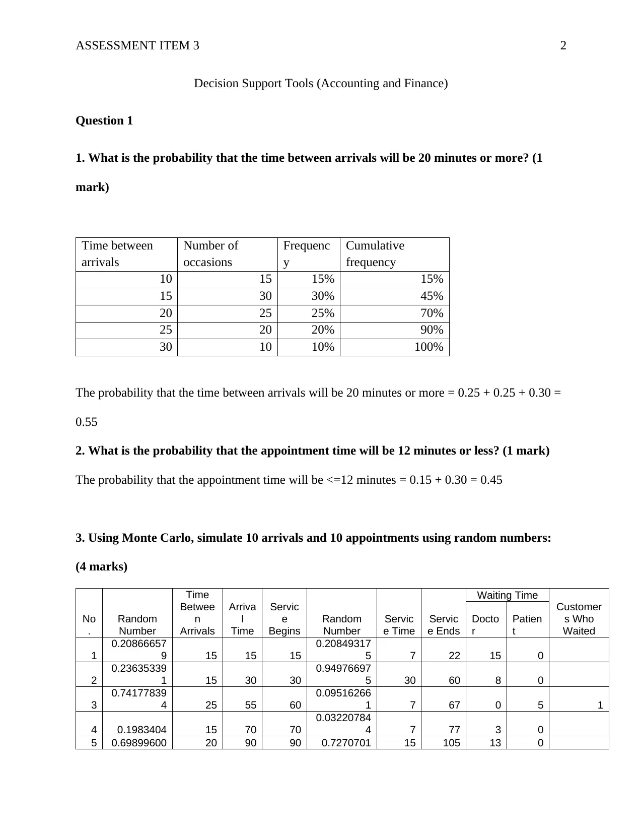
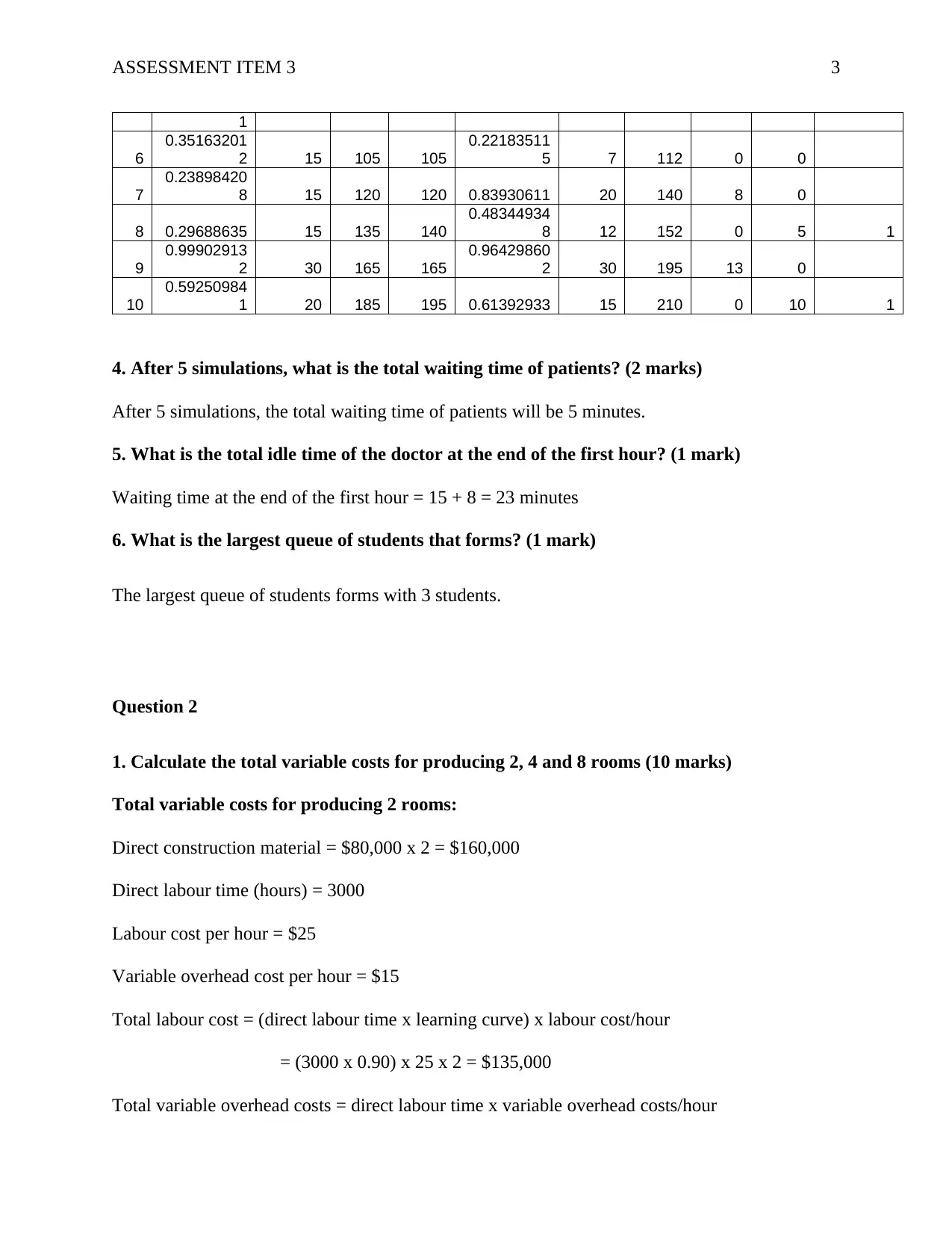
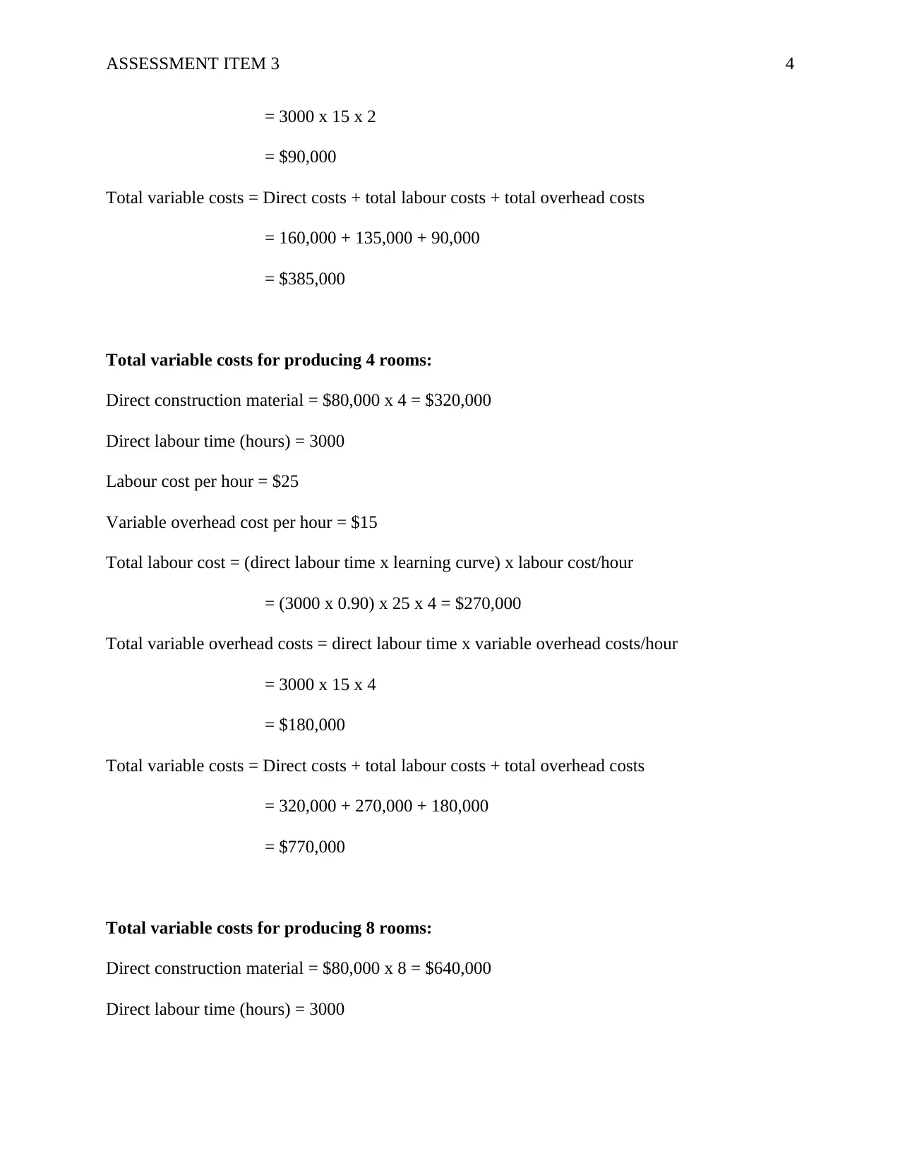
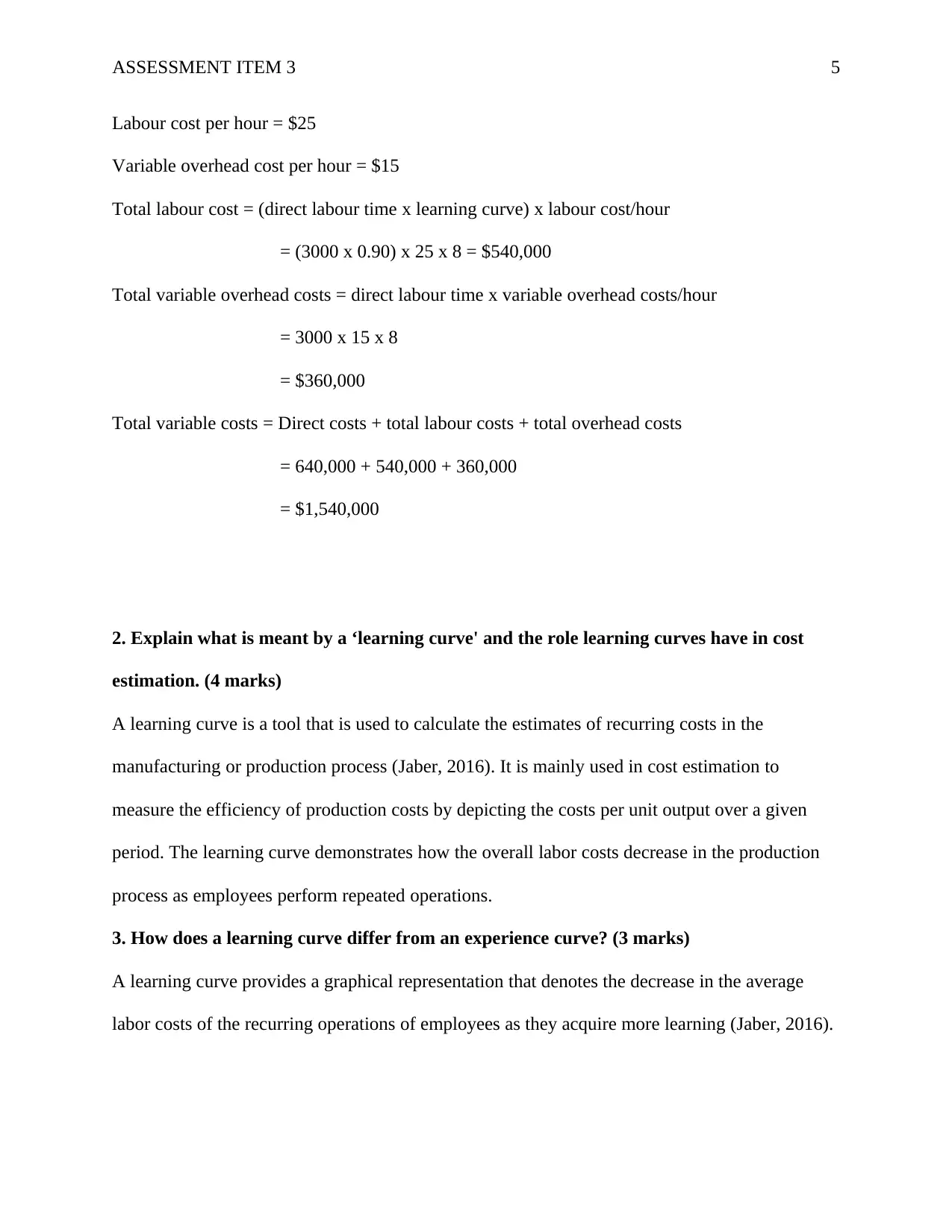
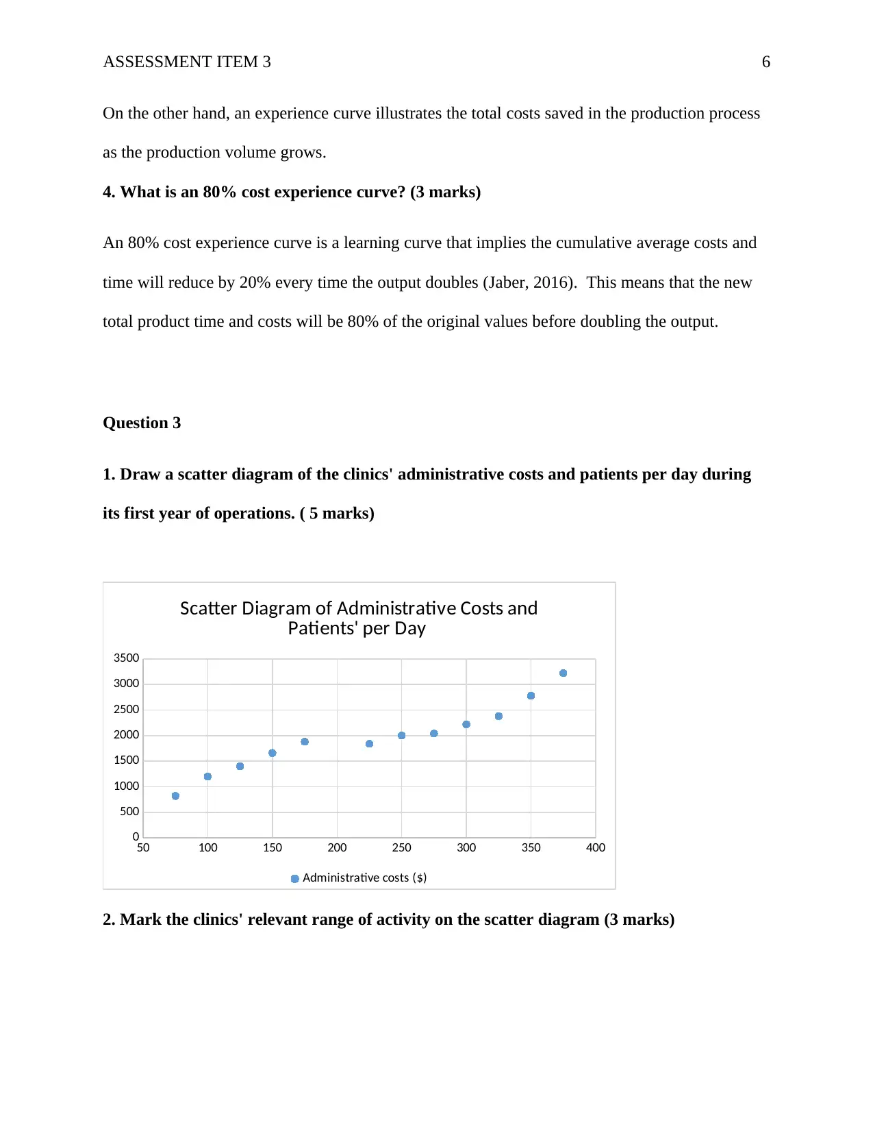
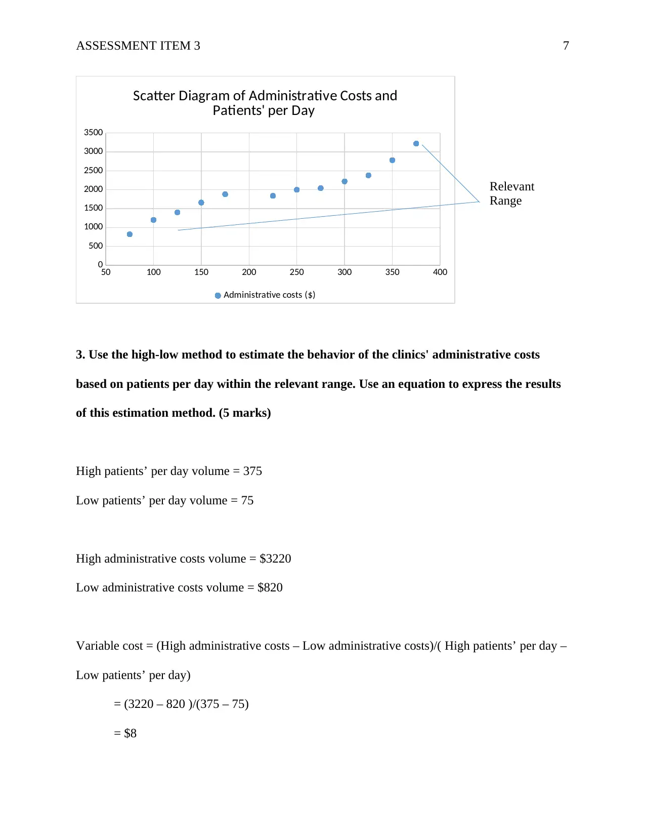
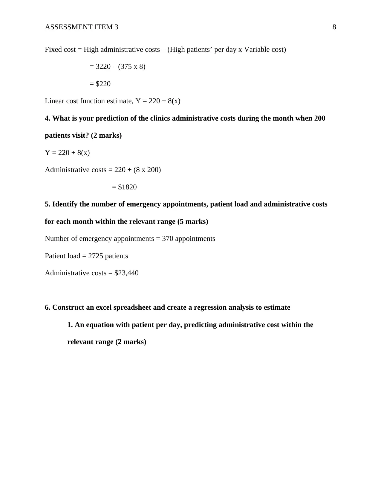
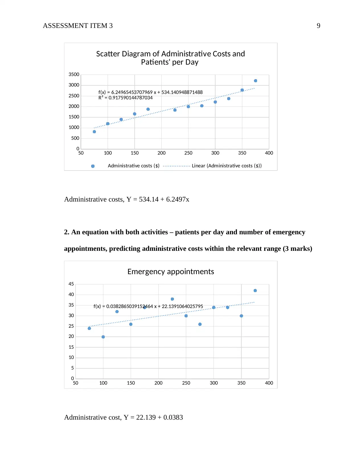
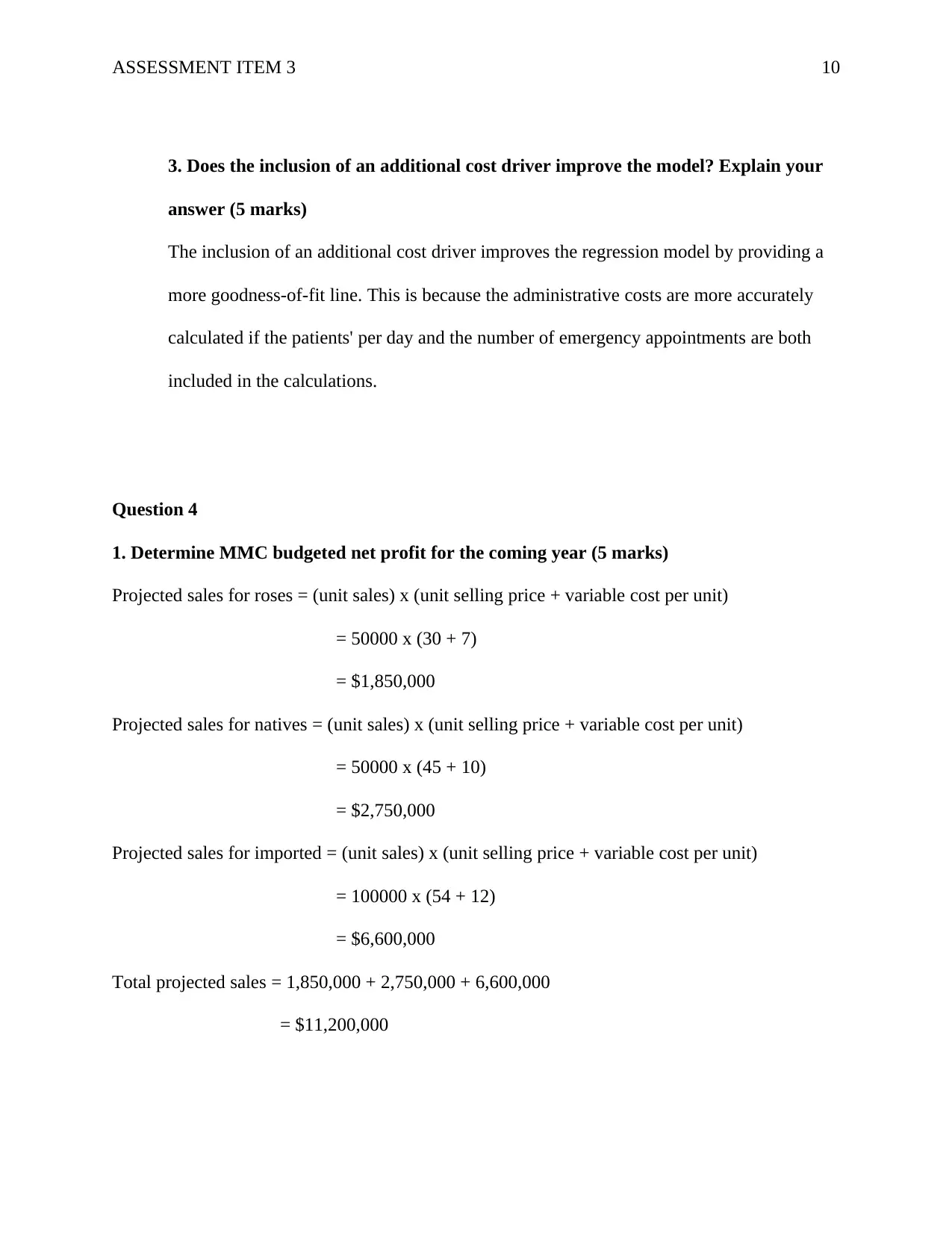
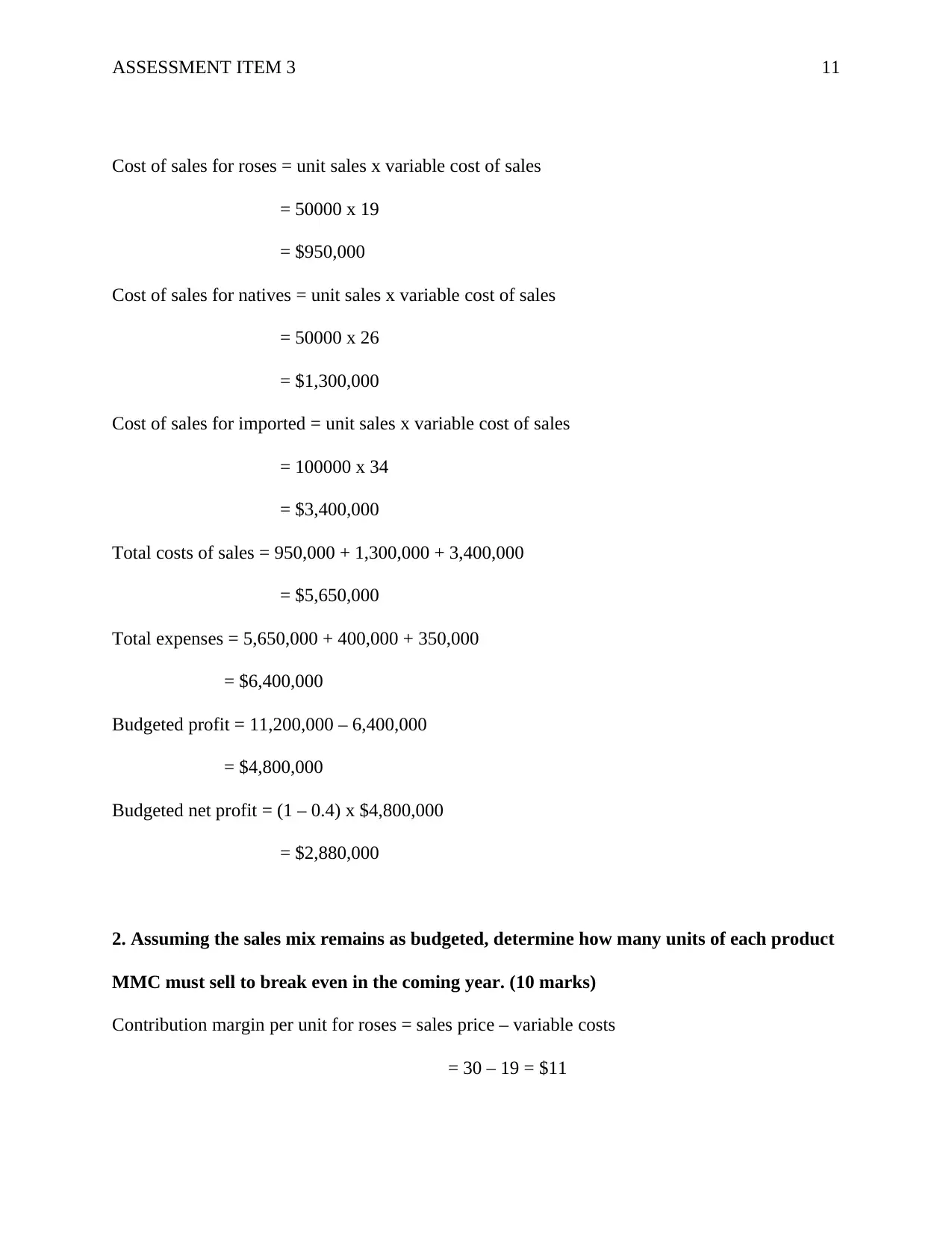
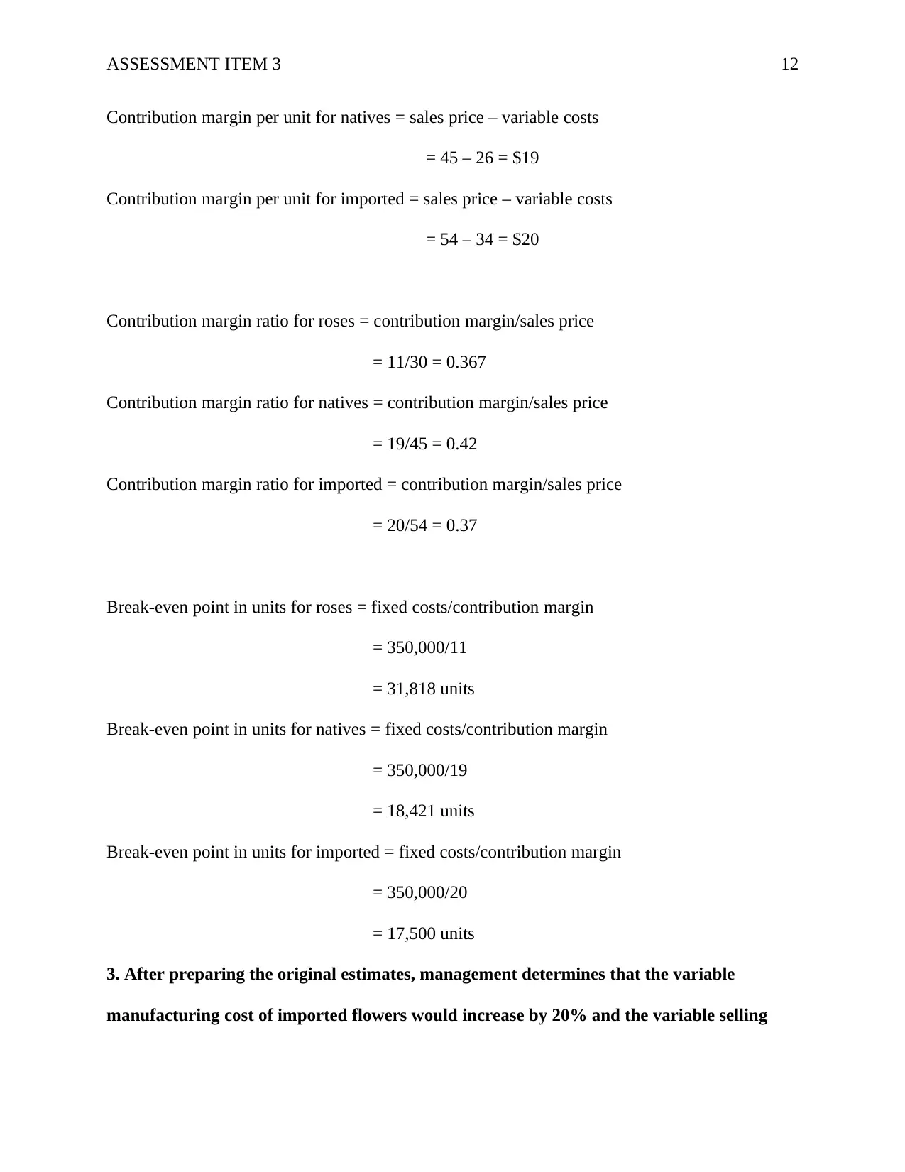
This assignment solution for ACC544, Decision Support Tools, addresses several key areas of finance and decision-making. Question 1 focuses on queuing theory and Monte Carlo simulation, involving probability calculations and simulating arrivals and appointments to analyze waiting times and idle time. Question 2 delves into cost accounting, requiring the calculation of variable costs, an explanation of learning and experience curves, and their role in cost estimation, including an 80% cost experience curve. Question 3 applies regression analysis to estimate administrative costs based on patient volume, employing the high-low method and creating a scatter diagram. It also predicts costs and uses regression models to analyze the impact of additional cost drivers. Question 4 deals with financial planning, including budgeting, break-even analysis, and the impact of changing costs and sales mix on profitability. The solution includes determining a budgeted net profit, calculating break-even points under different scenarios, and providing a memo to management with recommendations. The assignment covers a range of topics including simulation, cost accounting, regression, and financial planning, providing a comprehensive overview of decision support tools in a financial context.

Running head: ASSESSMENT ITEM 3 1
Assessment Item 3
Student name
Institutional affiliation

ASSESSMENT ITEM 3 2
Decision Support Tools (Accounting and Finance)
Question 1
1. What is the probability that the time between arrivals will be 20 minutes or more? (1
mark)
Time between
arrivals
Number of
occasions
Frequenc
y
Cumulative
frequency
10 15 15% 15%
15 30 30% 45%
20 25 25% 70%
25 20 20% 90%
30 10 10% 100%
The probability that the time between arrivals will be 20 minutes or more = 0.25 + 0.25 + 0.30 =
0.55
2. What is the probability that the appointment time will be 12 minutes or less? (1 mark)
The probability that the appointment time will be <=12 minutes = 0.15 + 0.30 = 0.45
3. Using Monte Carlo, simulate 10 arrivals and 10 appointments using random numbers:
(4 marks)
No
.
Random
Number
Time
Betwee
n
Arrivals
Arriva
l
Time
Servic
e
Begins
Random
Number
Servic
e Time
Servic
e Ends
Waiting Time
Customer
s Who
Waited
Docto
r
Patien
t
1
0.20866657
9 15 15 15
0.20849317
5 7 22 15 0
2
0.23635339
1 15 30 30
0.94976697
5 30 60 8 0
3
0.74177839
4 25 55 60
0.09516266
1 7 67 0 5 1
4 0.1983404 15 70 70
0.03220784
4 7 77 3 0
5 0.69899600 20 90 90 0.7270701 15 105 13 0

ASSESSMENT ITEM 3 3
1
6
0.35163201
2 15 105 105
0.22183511
5 7 112 0 0
7
0.23898420
8 15 120 120 0.83930611 20 140 8 0
8 0.29688635 15 135 140
0.48344934
8 12 152 0 5 1
9
0.99902913
2 30 165 165
0.96429860
2 30 195 13 0
10
0.59250984
1 20 185 195 0.61392933 15 210 0 10 1
4. After 5 simulations, what is the total waiting time of patients? (2 marks)
After 5 simulations, the total waiting time of patients will be 5 minutes.
5. What is the total idle time of the doctor at the end of the first hour? (1 mark)
Waiting time at the end of the first hour = 15 + 8 = 23 minutes
6. What is the largest queue of students that forms? (1 mark)
The largest queue of students forms with 3 students.
Question 2
1. Calculate the total variable costs for producing 2, 4 and 8 rooms (10 marks)
Total variable costs for producing 2 rooms:
Direct construction material = $80,000 x 2 = $160,000
Direct labour time (hours) = 3000
Labour cost per hour = $25
Variable overhead cost per hour = $15
Total labour cost = (direct labour time x learning curve) x labour cost/hour
= (3000 x 0.90) x 25 x 2 = $135,000
Total variable overhead costs = direct labour time x variable overhead costs/hour

ASSESSMENT ITEM 3 4
= 3000 x 15 x 2
= $90,000
Total variable costs = Direct costs + total labour costs + total overhead costs
= 160,000 + 135,000 + 90,000
= $385,000
Total variable costs for producing 4 rooms:
Direct construction material = $80,000 x 4 = $320,000
Direct labour time (hours) = 3000
Labour cost per hour = $25
Variable overhead cost per hour = $15
Total labour cost = (direct labour time x learning curve) x labour cost/hour
= (3000 x 0.90) x 25 x 4 = $270,000
Total variable overhead costs = direct labour time x variable overhead costs/hour
= 3000 x 15 x 4
= $180,000
Total variable costs = Direct costs + total labour costs + total overhead costs
= 320,000 + 270,000 + 180,000
= $770,000
Total variable costs for producing 8 rooms:
Direct construction material = $80,000 x 8 = $640,000
Direct labour time (hours) = 3000

ASSESSMENT ITEM 3 5
Labour cost per hour = $25
Variable overhead cost per hour = $15
Total labour cost = (direct labour time x learning curve) x labour cost/hour
= (3000 x 0.90) x 25 x 8 = $540,000
Total variable overhead costs = direct labour time x variable overhead costs/hour
= 3000 x 15 x 8
= $360,000
Total variable costs = Direct costs + total labour costs + total overhead costs
= 640,000 + 540,000 + 360,000
= $1,540,000
2. Explain what is meant by a ‘learning curve' and the role learning curves have in cost
estimation. (4 marks)
A learning curve is a tool that is used to calculate the estimates of recurring costs in the
manufacturing or production process (Jaber, 2016). It is mainly used in cost estimation to
measure the efficiency of production costs by depicting the costs per unit output over a given
period. The learning curve demonstrates how the overall labor costs decrease in the production
process as employees perform repeated operations.
3. How does a learning curve differ from an experience curve? (3 marks)
A learning curve provides a graphical representation that denotes the decrease in the average
labor costs of the recurring operations of employees as they acquire more learning (Jaber, 2016).

ASSESSMENT ITEM 3 6
On the other hand, an experience curve illustrates the total costs saved in the production process
as the production volume grows.
4. What is an 80% cost experience curve? (3 marks)
An 80% cost experience curve is a learning curve that implies the cumulative average costs and
time will reduce by 20% every time the output doubles (Jaber, 2016). This means that the new
total product time and costs will be 80% of the original values before doubling the output.
Question 3
1. Draw a scatter diagram of the clinics' administrative costs and patients per day during
its first year of operations. ( 5 marks)
50 100 150 200 250 300 350 400
0
500
1000
1500
2000
2500
3000
3500
Scatter Diagram of Administrative Costs and
Patients' per Day
Administrative costs ($)
2. Mark the clinics' relevant range of activity on the scatter diagram (3 marks)

ASSESSMENT ITEM 3 7
50 100 150 200 250 300 350 400
0
500
1000
1500
2000
2500
3000
3500
Scatter Diagram of Administrative Costs and
Patients' per Day
Administrative costs ($)
3. Use the high-low method to estimate the behavior of the clinics' administrative costs
based on patients per day within the relevant range. Use an equation to express the results
of this estimation method. (5 marks)
High patients’ per day volume = 375
Low patients’ per day volume = 75
High administrative costs volume = $3220
Low administrative costs volume = $820
Variable cost = (High administrative costs – Low administrative costs)/( High patients’ per day –
Low patients’ per day)
= (3220 – 820 )/(375 – 75)
= $8
Relevant
Range

ASSESSMENT ITEM 3 8
Fixed cost = High administrative costs – (High patients’ per day x Variable cost)
= 3220 – (375 x 8)
= $220
Linear cost function estimate, Y = 220 + 8(x)
4. What is your prediction of the clinics administrative costs during the month when 200
patients visit? (2 marks)
Y = 220 + 8(x)
Administrative costs = 220 + (8 x 200)
= $1820
5. Identify the number of emergency appointments, patient load and administrative costs
for each month within the relevant range (5 marks)
Number of emergency appointments = 370 appointments
Patient load = 2725 patients
Administrative costs = $23,440
6. Construct an excel spreadsheet and create a regression analysis to estimate
1. An equation with patient per day, predicting administrative cost within the
relevant range (2 marks)

ASSESSMENT ITEM 3 9
50 100 150 200 250 300 350 400
0
500
1000
1500
2000
2500
3000
3500
f(x) = 6.24965453707969 x + 534.140948871488
R² = 0.917590144787034
Scatter Diagram of Administrative Costs and
Patients' per Day
Administrative costs ($) Linear (Administrative costs ($))
Administrative costs, Y = 534.14 + 6.2497x
2. An equation with both activities – patients per day and number of emergency
appointments, predicting administrative costs within the relevant range (3 marks)
50 100 150 200 250 300 350 400
0
5
10
15
20
25
30
35
40
45
f(x) = 0.0382865039152464 x + 22.1391064025795
Emergency appointments
Administrative cost, Y = 22.139 + 0.0383

ASSESSMENT ITEM 3 10
3. Does the inclusion of an additional cost driver improve the model? Explain your
answer (5 marks)
The inclusion of an additional cost driver improves the regression model by providing a
more goodness-of-fit line. This is because the administrative costs are more accurately
calculated if the patients' per day and the number of emergency appointments are both
included in the calculations.
Question 4
1. Determine MMC budgeted net profit for the coming year (5 marks)
Projected sales for roses = (unit sales) x (unit selling price + variable cost per unit)
= 50000 x (30 + 7)
= $1,850,000
Projected sales for natives = (unit sales) x (unit selling price + variable cost per unit)
= 50000 x (45 + 10)
= $2,750,000
Projected sales for imported = (unit sales) x (unit selling price + variable cost per unit)
= 100000 x (54 + 12)
= $6,600,000
Total projected sales = 1,850,000 + 2,750,000 + 6,600,000
= $11,200,000

ASSESSMENT ITEM 3 11
Cost of sales for roses = unit sales x variable cost of sales
= 50000 x 19
= $950,000
Cost of sales for natives = unit sales x variable cost of sales
= 50000 x 26
= $1,300,000
Cost of sales for imported = unit sales x variable cost of sales
= 100000 x 34
= $3,400,000
Total costs of sales = 950,000 + 1,300,000 + 3,400,000
= $5,650,000
Total expenses = 5,650,000 + 400,000 + 350,000
= $6,400,000
Budgeted profit = 11,200,000 – 6,400,000
= $4,800,000
Budgeted net profit = (1 – 0.4) x $4,800,000
= $2,880,000
2. Assuming the sales mix remains as budgeted, determine how many units of each product
MMC must sell to break even in the coming year. (10 marks)
Contribution margin per unit for roses = sales price – variable costs
= 30 – 19 = $11

ASSESSMENT ITEM 3 12
Contribution margin per unit for natives = sales price – variable costs
= 45 – 26 = $19
Contribution margin per unit for imported = sales price – variable costs
= 54 – 34 = $20
Contribution margin ratio for roses = contribution margin/sales price
= 11/30 = 0.367
Contribution margin ratio for natives = contribution margin/sales price
= 19/45 = 0.42
Contribution margin ratio for imported = contribution margin/sales price
= 20/54 = 0.37
Break-even point in units for roses = fixed costs/contribution margin
= 350,000/11
= 31,818 units
Break-even point in units for natives = fixed costs/contribution margin
= 350,000/19
= 18,421 units
Break-even point in units for imported = fixed costs/contribution margin
= 350,000/20
= 17,500 units
3. After preparing the original estimates, management determines that the variable
manufacturing cost of imported flowers would increase by 20% and the variable selling

ASSESSMENT ITEM 3 13
cost of natives could be expected to increase by $3.00 per units. However, management has
decided not to change the selling price of either product. Also, management has learned
that imported flowers are perceived to be the best value for money, and they can expect to
sell three times as many imported flowers as each of their other products. Under these
circumstances, determine how many units of each product MMC would have to sell to
break even in the coming year. (10 marks)
Contribution margin per unit for roses = sales price – variable costs
= 30 – 19 = $11
Contribution margin per unit for natives = sales price – variable costs
= 45 – 29 = $16
Contribution margin per unit for imported = sales price – variable costs
= 54 – 40.8 = $13.2
Contribution margin ratio for roses = contribution margin/sales price
= 11/30 = 0.367
Contribution margin ratio for natives = contribution margin/sales price
= 16/45 = 0.36
Contribution margin ratio for imported = contribution margin/sales price
= 13.2/54 = 0.24
Break-even point in units for roses = fixed costs/contribution margin
= 350,000/11
= 31,818 units

ASSESSMENT ITEM 3 14
Break-even point in units for natives = fixed costs/contribution margin
= 350,000/16
= 21,875 units
Break-even point in units for imported = fixed costs/contribution margin
= 350,000/13.2
= 26,515 units
4. Write a one-page memo to management, recommending what action they should take, as
determined in Parts 2 and 3. Justify your choice. (5 marks)
Memorandum
TO: Mediocre Medical Centre Management
FROM: Student name
DATE: 22/9/2019
SUBJECT: Recommended actions regarding Sale of Flowers
It has come to my notice that the company is interested in building a florist in the medical center.
This memorandum is hereby addressed to the Mediocre Medical Centre manages in concern to
the sale of the flowers. The company intends to sale three main varieties of flowers comprising
roses, natives, and imported flowers. From the analysis carried out, it is noted that flowers vary
in terms of the sales prices and variable prices. To generate profit from the business, the MMC
management needs to consider the sales volume of the flowers and the forecasted variable prices
of each flower categories.
From the analysis, the management should consider the following volumes that will be essential
in attaining a break-even point in the coming year:
 Sale 31,818 units of rose flowers

ASSESSMENT ITEM 3 15
 Sale 18,421 units of native flowers
 Sale 17,500 units of imported flowers
However, considering the fluctuations in the market, variable costs for manufacturing are subject
to rising by 20% and the variable selling cost of natives will rise by $3.00 per unit. The
management considers selling imported flowers due to high market prices. Conversely, the
analysis indicates that management will have to sell more units of imported flowers if they are to
reach a break-even point in the coming year. Therefore, it is recommended that the management
sticks to the previous prices rather than adopting the new changes. This will enable the company
to attain breakeven point with fewer units of imported flowers than in the proposed changes.
Yours faithfully,
Student name
Question 5
1. Describe what qualitative forecasting models are. What are the advantages and
disadvantages of this modeling? (5 marks)
Qualitative forecasting models are the predictive techniques that are subjective on the
opinions of consumers as well as experts (Degiannakis & Floros, 2016). These models are
appropriate in situations where there is no data figure to be used in the modeling of situations.
The advantages of qualitative forecasting include the ability to forecast changes in customer
behaviors and sales patterns by considering expert judgment, ease of flexibility in predictions,

ASSESSMENT ITEM 3 16
and useful in forecasting in situations with ambiguous data. On the other hand, the disadvantages
include anchoring of events, selected perceptions, provision of inaccurate forecasts, and reliance
on forecaster biases.
2. “High correlation between two variables means that one is the cause and the other is the
effect”. Explain this statement (5 marks)
The high correlation between two variables implies that one is the causal variable while
the other is the effective variable (Degiannakis & Floros, 2016). This statement means that two
variables with high correlation degree have a driving force between them. The causal variable is
considered to be the independent variable and the other which feels the effects is the dependent
variable. Therefore, to have a high correlation between two variable, the two must have some
dependence.