Comprehensive Analysis of Decision Support Tools in Finance

This assignment delves into the application of various decision support tools within a financial context. It begins with an exploration of decision analysis, including assessing utility functions and standard gamble techniques to evaluate investment scenarios in the share market. The assignment then covers the value of information, analyzing prior and posterior probabilities to determine expected net gains and losses from market research. Monte Carlo simulation and regression analysis are also employed to evaluate different financial models. Furthermore, the assignment uses CVP (Cost-Volume-Profit) analysis to determine break-even points and contribution margins for different products. The solution provides detailed calculations and explanations for each section, offering a comprehensive understanding of these crucial financial decision-making tools.

Decision Support Tools

TABLE OF CONTENTS
QUESTION 1: DECISION ANALYSIS.........................................................................................4
A. Assessing the utility function as well as standard gamble which helps in determining utility
value.............................................................................................................................................4
B. Investing primarily in share market........................................................................................4
1...................................................................................................................................................4
2...................................................................................................................................................5
3...................................................................................................................................................5
4...................................................................................................................................................5
5...................................................................................................................................................5
6...................................................................................................................................................5
QUESTION 2: VALUE OF INFORMATION................................................................................6
a....................................................................................................................................................6
B. Analyzing the prior probability...............................................................................................6
C. Posterior probability................................................................................................................7
D. Expected net gain and loss after conducting the market research..........................................7
QUESTION 3 MONTE CARLO SIMULATION...........................................................................7
a....................................................................................................................................................7
b...................................................................................................................................................7
QUESTION 4 REGRESSION ANALYSIS....................................................................................8
a....................................................................................................................................................8
b...................................................................................................................................................8
c..................................................................................................................................................12
d.................................................................................................................................................12
QUESTION 5: CVP ANALYSIS..................................................................................................13

a..................................................................................................................................................13
b.................................................................................................................................................13
c..................................................................................................................................................14
d.................................................................................................................................................14
D (i)............................................................................................................................................14
D (ii)...........................................................................................................................................14

QUESTION 1: DECISION ANALYSIS
A. Assessing the utility function as well as standard gamble which helps in determining utility
value
In utility assessment, it consists of identifying bad and best utility to be used in process.
Thus, where 0 represents a bad, while 1 for good quality of a utility. This assessment helps in
ranking the commodities which will be helpful in identifying no. of better and worst articles are
stated in a study. In context with implicating this theory which determines that, monetary value
will not be a reliable indication in judging over all outcomes and make decision. Here,
economists have to assume that significant individual makes decision to enhance their utilities.
Standard Gamble:
In consideration with this approach the standard gamble techniques had been used in
analyzing the values of utilities. It assists that when the variables are indifferent the utility values
are equal.
B. Investing primarily in share market
1.
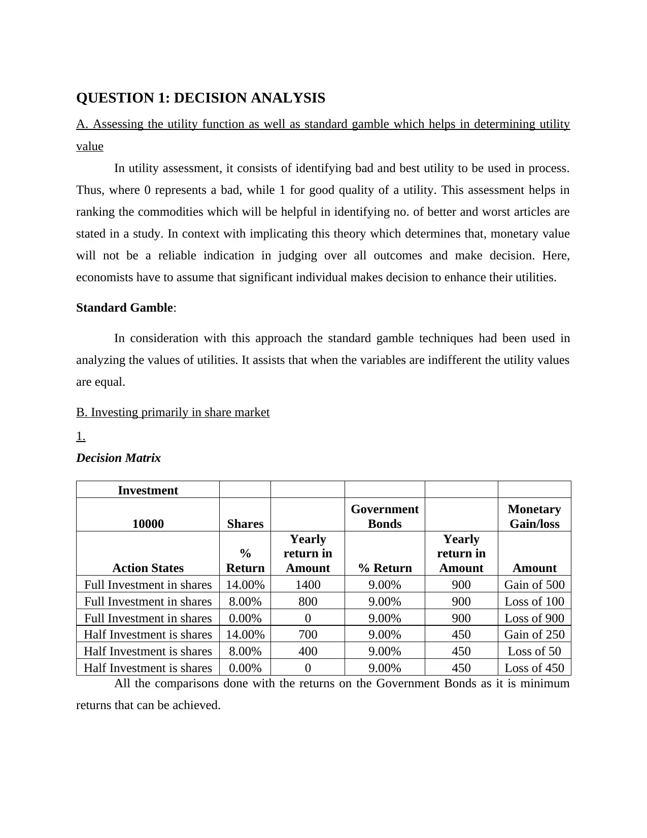
Decision Matrix
Investment
10000 Shares
Government
Bonds
Monetary
Gain/loss
Action States
%
Return
Yearly
return in
Amount % Return
Yearly
return in
Amount Amount
Full Investment in shares 14.00% 1400 9.00% 900 Gain of 500
Full Investment in shares 8.00% 800 9.00% 900 Loss of 100
Full Investment in shares 0.00% 0 9.00% 900 Loss of 900
Half Investment is shares 14.00% 700 9.00% 450 Gain of 250
Half Investment is shares 8.00% 400 9.00% 450 Loss of 50
Half Investment is shares 0.00% 0 9.00% 450 Loss of 450
All the comparisons done with the returns on the Government Bonds as it is minimum
returns that can be achieved.

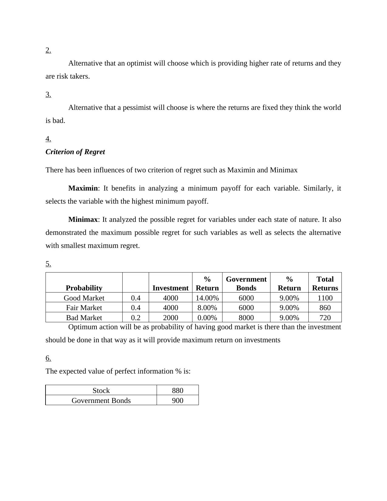
2.
Alternative that an optimist will choose which is providing higher rate of returns and they
are risk takers.
3.
Alternative that a pessimist will choose is where the returns are fixed they think the world
is bad.
4.
Criterion of Regret
There has been influences of two criterion of regret such as Maximin and Minimax
Maximin: It benefits in analyzing a minimum payoff for each variable. Similarly, it
selects the variable with the highest minimum payoff.
Minimax: It analyzed the possible regret for variables under each state of nature. It also
demonstrated the maximum possible regret for such variables as well as selects the alternative
with smallest maximum regret.
5.
Probability Investment
%
Return
Government
Bonds
%
Return
Total
Returns
Good Market 0.4 4000 14.00% 6000 9.00% 1100
Fair Market 0.4 4000 8.00% 6000 9.00% 860
Bad Market 0.2 2000 0.00% 8000 9.00% 720
Optimum action will be as probability of having good market is there than the investment
should be done in that way as it will provide maximum return on investments
6.
The expected value of perfect information % is:
Stock 880
Government Bonds 900

As the maximum of expectation is in Government Bonds. As not knowing the directions
where will be the market go we expect the most of returns from government bonds thus EMV
=900
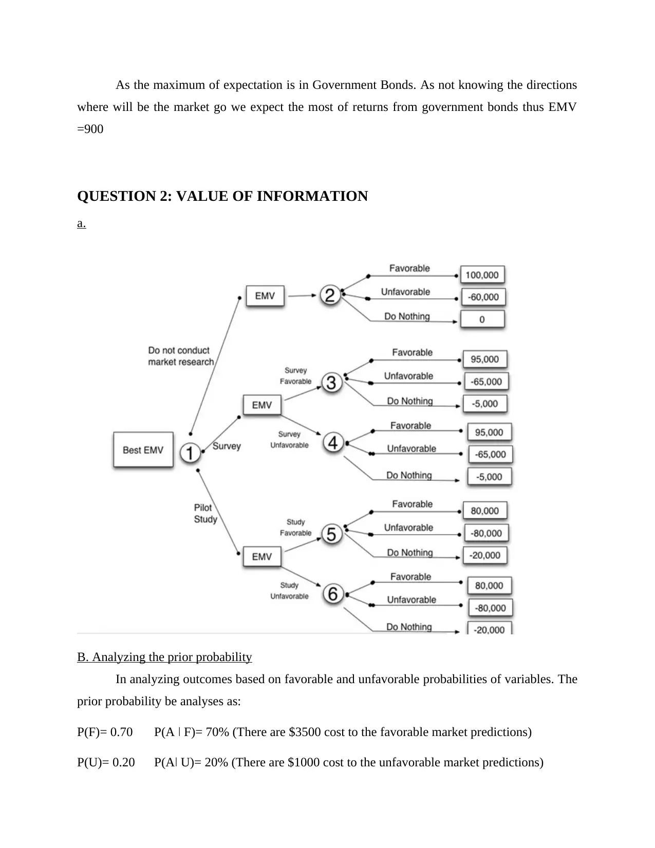
QUESTION 2: VALUE OF INFORMATION
a.
B. Analyzing the prior probability
In analyzing outcomes based on favorable and unfavorable probabilities of variables. The
prior probability be analyses as:
P(F)= 0.70 P(A ǀ F)= 70% (There are $3500 cost to the favorable market predictions)
P(U)= 0.20 P(Aǀ U)= 20% (There are $1000 cost to the unfavorable market predictions)

C. Posterior probability
P(A) = P(A ǀ F) P(F) + P(A ǀ U) P(U)
P(F ǀ A) = P(F ∩ A)/P(A) = P(A ǀ F) P(F)/P(A ǀ F) P(M) + P(A ǀ U) P(U)
= 3500*0.7 / (3500*0.7) + (1000*0.2)
= 0.924
P(U ǀ A) = P(U ∩ A)/ P(A) = P(A ǀ U) P(U)/ P(A ǀ F) P(F) + P(A ǀ U) P(U)
1000* 0.20/ (3500*0.7)+ (1000*0.2)
= 0.075
D. Expected net gain and loss after conducting the market research
Probability of having favorable outcomes = 3500
Probability of having unfavorable outcomes are = 1000
Therefore,
=3500-1000
= 2500
There will be gain of 2500 which insist that the market research will be helpful in bringing the
suitable gains.
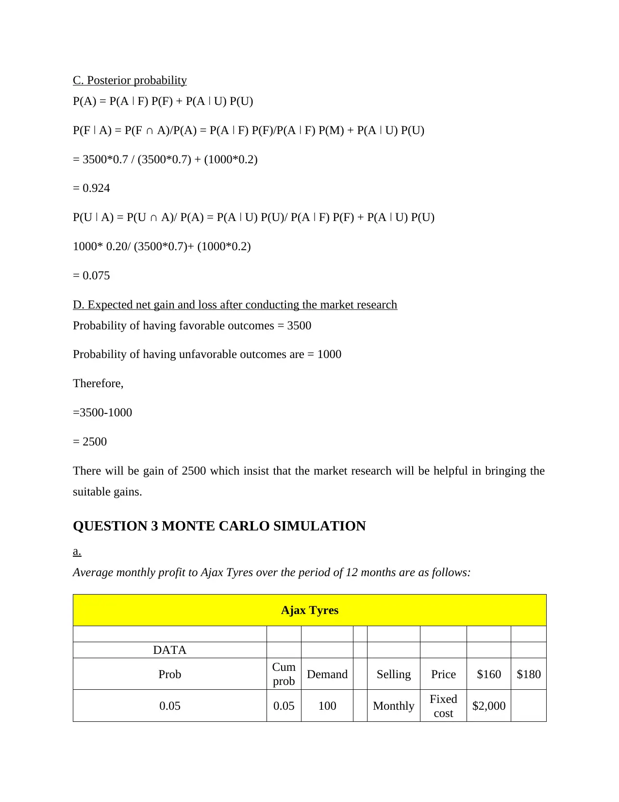
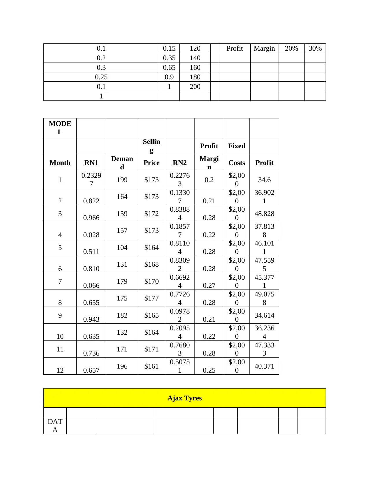
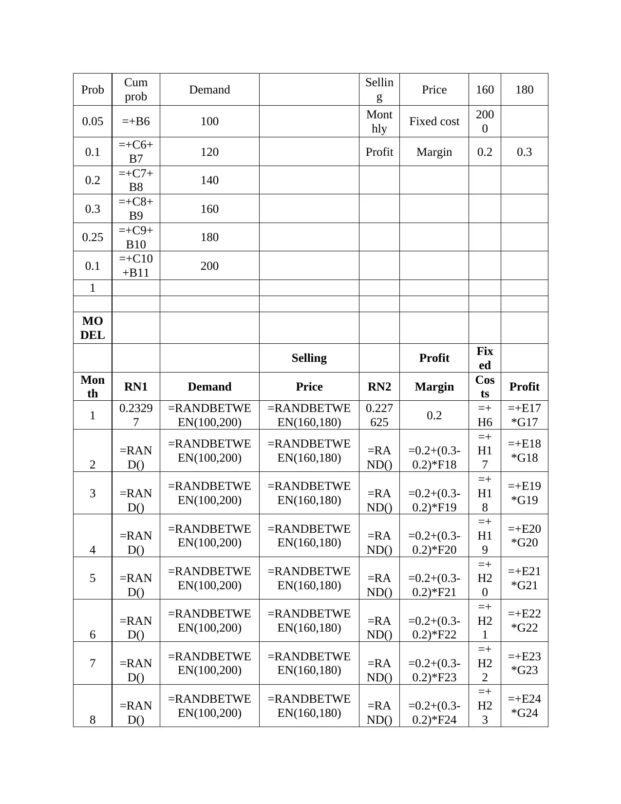
QUESTION 3 MONTE CARLO SIMULATION
a.
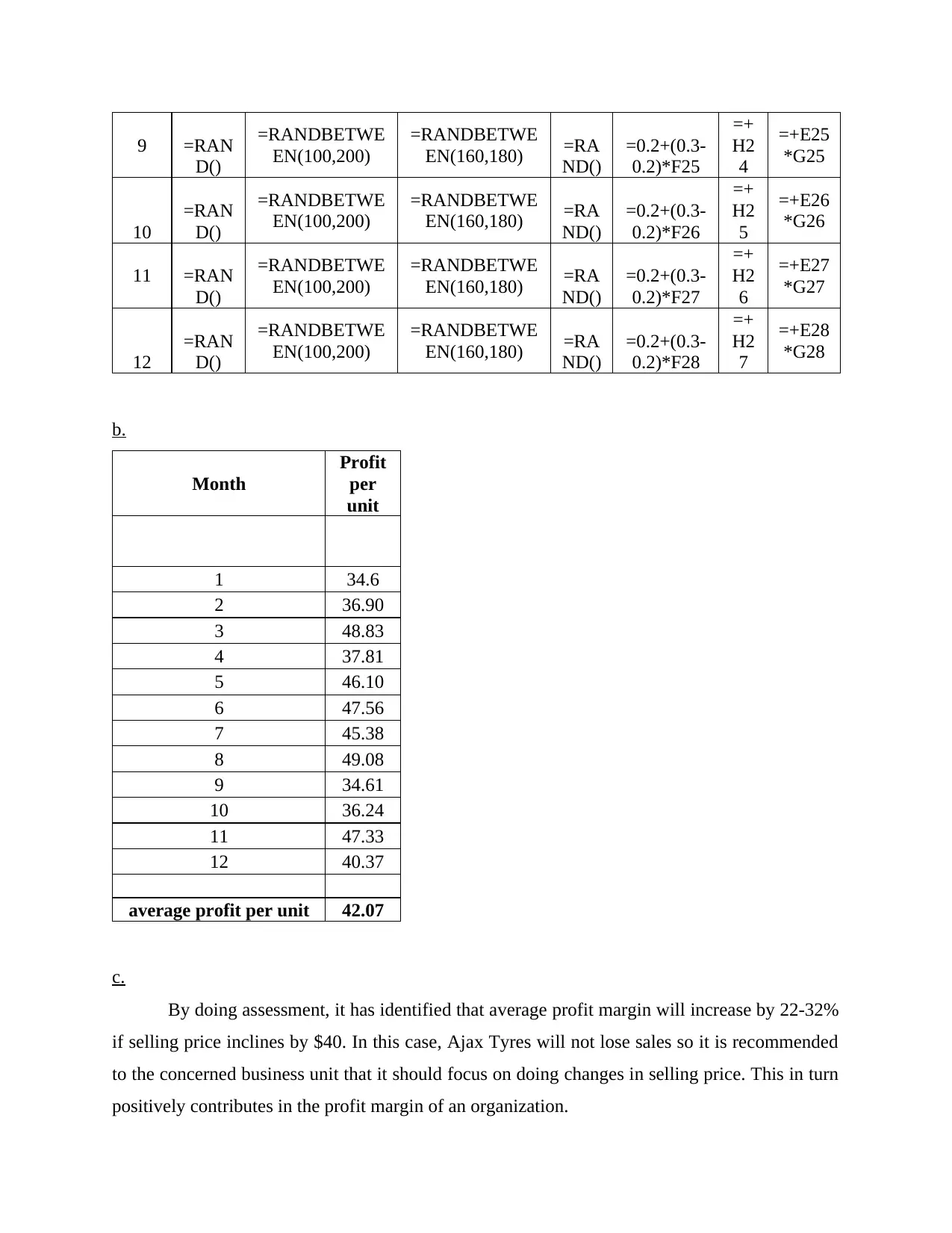
Average monthly profit to Ajax Tyres over the period of 12 months are as follows:
Ajax Tyres
DATA
Prob Cum
prob Demand Selling Price $160 $180
0.05 0.05 100 Monthly Fixed
cost $2,000

0.1 0.15 120 Profit Margin 20% 30%
0.2 0.35 140
0.3 0.65 160
0.25 0.9 180
0.1 1 200
1
MODE
L
Sellin
g Profit Fixed
Month RN1 Deman
d Price RN2 Margi
n Costs Profit
1 0.2329
7 199 $173 0.2276
3 0.2 $2,00
0 34.6
2 0.822 164 $173 0.1330
7 0.21
$2,00
0
36.902
1
3 0.966 159 $172 0.8388
4 0.28
$2,00
0 48.828
4 0.028 157 $173 0.1857
7 0.22
$2,00
0
37.813
8
5 0.511 104 $164 0.8110
4 0.28
$2,00
0
46.101
1
6 0.810 131 $168 0.8309
2 0.28
$2,00
0
47.559
5
7 0.066 179 $170 0.6692
4 0.27
$2,00
0
45.377
1
8 0.655 175 $177 0.7726
4 0.28
$2,00
0
49.075
8
9 0.943 182 $165 0.0978
2 0.21
$2,00
0 34.614
10 0.635 132 $164 0.2095
4 0.22
$2,00
0
36.236
4
11 0.736 171 $171 0.7680
3 0.28
$2,00
0
47.333
3
12 0.657 196 $161 0.5075
1 0.25
$2,00
0 40.371
Ajax Tyres
DAT
A

Prob Cum
prob Demand Sellin
g Price 160 180
0.05 =+B6 100 Mont
hly Fixed cost 200
0
0.1 =+C6+
B7 120 Profit Margin 0.2 0.3
0.2 =+C7+
B8 140
0.3 =+C8+
B9 160
0.25 =+C9+
B10 180
0.1 =+C10
+B11 200
1
MO
DEL
Selling Profit Fix
ed
Mon
th RN1 Demand Price RN2 Margin Cos
ts Profit
1 0.2329
7
=RANDBETWE
EN(100,200)
=RANDBETWE
EN(160,180)
0.227
625 0.2 =+
H6
=+E17
*G17
2
=RAN
D()
=RANDBETWE
EN(100,200)
=RANDBETWE
EN(160,180) =RA
ND()
=0.2+(0.3-
0.2)*F18
=+
H1
7
=+E18
*G18
3 =RAN
D()
=RANDBETWE
EN(100,200)
=RANDBETWE
EN(160,180) =RA
ND()
=0.2+(0.3-
0.2)*F19
=+
H1
8
=+E19
*G19
4
=RAN
D()
=RANDBETWE
EN(100,200)
=RANDBETWE
EN(160,180) =RA
ND()
=0.2+(0.3-
0.2)*F20
=+
H1
9
=+E20
*G20
5 =RAN
D()
=RANDBETWE
EN(100,200)
=RANDBETWE
EN(160,180) =RA
ND()
=0.2+(0.3-
0.2)*F21
=+
H2
0
=+E21
*G21
6
=RAN
D()
=RANDBETWE
EN(100,200)
=RANDBETWE
EN(160,180) =RA
ND()
=0.2+(0.3-
0.2)*F22
=+
H2
1
=+E22
*G22
7 =RAN
D()
=RANDBETWE
EN(100,200)
=RANDBETWE
EN(160,180) =RA
ND()
=0.2+(0.3-
0.2)*F23
=+
H2
2
=+E23
*G23
8
=RAN
D()
=RANDBETWE
EN(100,200)
=RANDBETWE
EN(160,180) =RA
ND()
=0.2+(0.3-
0.2)*F24
=+
H2
3
=+E24
*G24

9 =RAN
D()
=RANDBETWE
EN(100,200)
=RANDBETWE
EN(160,180) =RA
ND()
=0.2+(0.3-
0.2)*F25
=+
H2
4
=+E25
*G25
10
=RAN
D()
=RANDBETWE
EN(100,200)
=RANDBETWE
EN(160,180) =RA
ND()
=0.2+(0.3-
0.2)*F26
=+
H2
5
=+E26
*G26
11 =RAN
D()
=RANDBETWE
EN(100,200)
=RANDBETWE
EN(160,180) =RA
ND()
=0.2+(0.3-
0.2)*F27
=+
H2
6
=+E27
*G27
12
=RAN
D()
=RANDBETWE
EN(100,200)
=RANDBETWE
EN(160,180) =RA
ND()
=0.2+(0.3-
0.2)*F28
=+
H2
7
=+E28
*G28
b.
Month
Profit
per
unit
1 34.6
2 36.90
3 48.83
4 37.81
5 46.10
6 47.56
7 45.38
8 49.08
9 34.61
10 36.24
11 47.33
12 40.37
average profit per unit 42.07
c.
By doing assessment, it has identified that average profit margin will increase by 22-32%
if selling price inclines by $40. In this case, Ajax Tyres will not lose sales so it is recommended
to the concerned business unit that it should focus on doing changes in selling price. This in turn
positively contributes in the profit margin of an organization.

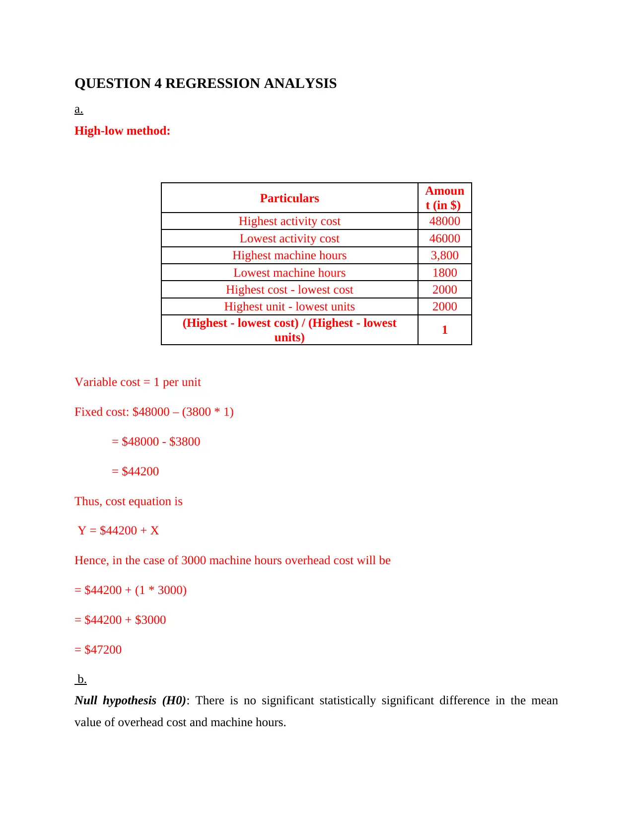
QUESTION 4 REGRESSION ANALYSIS
a.
High-low method:
Particulars Amoun
t (in $)
Highest activity cost 48000
Lowest activity cost 46000
Highest machine hours 3,800
Lowest machine hours 1800
Highest cost - lowest cost 2000
Highest unit - lowest units 2000
(Highest - lowest cost) / (Highest - lowest
units) 1
Variable cost = 1 per unit
Fixed cost: $48000 – (3800 * 1)
= $48000 - $3800
= $44200
Thus, cost equation is
Y = $44200 + X
Hence, in the case of 3000 machine hours overhead cost will be
= $44200 + (1 * 3000)
= $44200 + $3000
= $47200
b.
Null hypothesis (H0): There is no significant statistically significant difference in the mean
value of overhead cost and machine hours.

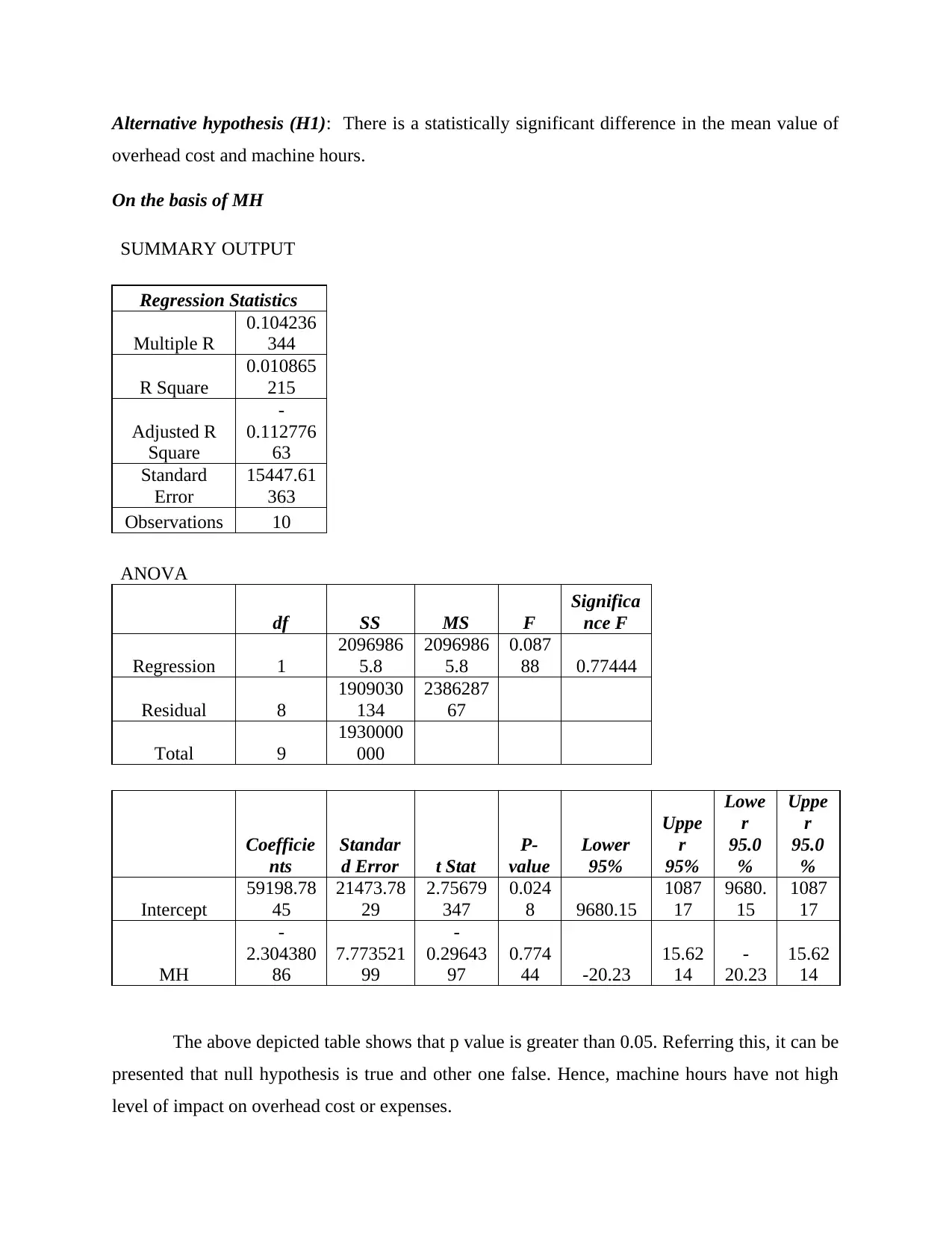
Alternative hypothesis (H1): There is a statistically significant difference in the mean value of
overhead cost and machine hours.
On the basis of MH
SUMMARY OUTPUT
Regression Statistics
Multiple R
0.104236
344
R Square
0.010865
215
Adjusted R
Square
-
0.112776
63
Standard
Error
15447.61
363
Observations 10
ANOVA
df SS MS F
Significa
nce F
Regression 1
2096986
5.8
2096986
5.8
0.087
88 0.77444
Residual 8
1909030
134
2386287
67
Total 9
1930000
000
Coefficie
nts
Standar
d Error t Stat
P-
value
Lower
95%
Uppe
r
95%
Lowe
r
95.0
%
Uppe
r
95.0
%
Intercept
59198.78
45
21473.78
29
2.75679
347
0.024
8 9680.15
1087
17
9680.
15
1087
17
MH
-
2.304380
86
7.773521
99
-
0.29643
97
0.774
44 -20.23
15.62
14
-
20.23
15.62
14
The above depicted table shows that p value is greater than 0.05. Referring this, it can be
presented that null hypothesis is true and other one false. Hence, machine hours have not high
level of impact on overhead cost or expenses.