RM Ltd. Finance Assignment: Income Statement and Balance Sheet
VerifiedAdded on 2022/11/24
|10
|2020
|413
Homework Assignment
AI Summary
This finance assignment solution addresses key concepts in financial accounting and management. It begins with the preparation of an income statement and statement of financial position for RM Ltd., incorporating adjustments for inventory valuation, accruals, depreciation, and taxation. The solution then delves into project appraisal, calculating payback periods and net present values for two projects, followed by a discussion of project ranking and additional factors influencing investment decisions. Finally, the assignment concludes with a breakeven analysis, calculating contribution margins, breakeven points, and margins of safety, while also addressing the limitations of breakeven analysis.

FINANCE
Paraphrase This Document
Need a fresh take? Get an instant paraphrase of this document with our AI Paraphraser

Table of Contents
Question: 1.......................................................................................................................................3
SECTION- B...................................................................................................................................5
QUESTION- 2.................................................................................................................................5
Question: 4.......................................................................................................................................8
REFERENCES..............................................................................................................................10
Question: 1
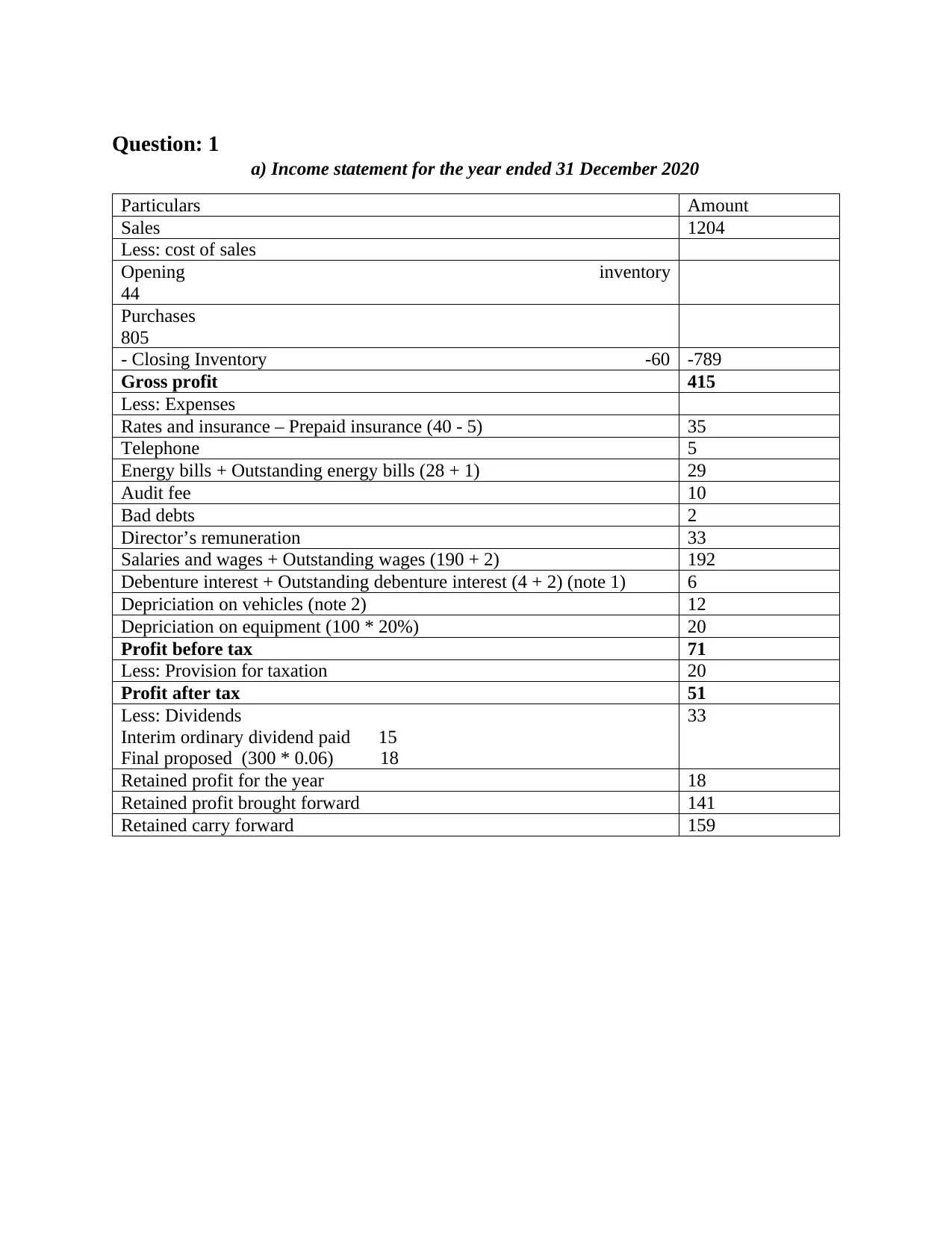
a) Income statement for the year ended 31 December 2020
Particulars Amount
Sales 1204
Less: cost of sales
Opening inventory
44
Purchases
805
- Closing Inventory -60 -789
Gross profit 415
Less: Expenses
Rates and insurance – Prepaid insurance (40 - 5) 35
Telephone 5
Energy bills + Outstanding energy bills (28 + 1) 29
Audit fee 10
Bad debts 2
Director’s remuneration 33
Salaries and wages + Outstanding wages (190 + 2) 192
Debenture interest + Outstanding debenture interest (4 + 2) (note 1) 6
Depriciation on vehicles (note 2) 12
Depriciation on equipment (100 * 20%) 20
Profit before tax 71
Less: Provision for taxation 20
Profit after tax 51
Less: Dividends
Interim ordinary dividend paid 15
Final proposed (300 * 0.06) 18
33
Retained profit for the year 18
Retained profit brought forward 141
Retained carry forward 159
⊘ This is a preview!⊘
Do you want full access?
Subscribe today to unlock all pages.
Trusted by 1+ million students worldwide
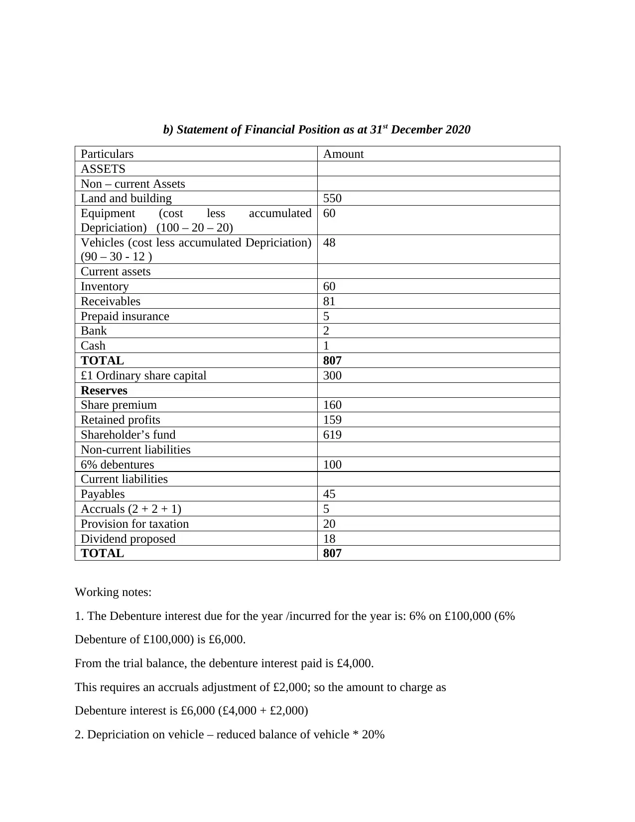
b) Statement of Financial Position as at 31st December 2020
Particulars Amount
ASSETS
Non – current Assets
Land and building 550
Equipment (cost less accumulated
Depriciation) (100 – 20 – 20)
60
Vehicles (cost less accumulated Depriciation)
(90 – 30 - 12 )
48
Current assets
Inventory 60
Receivables 81
Prepaid insurance 5
Bank 2
Cash 1
TOTAL 807
£1 Ordinary share capital 300
Reserves
Share premium 160
Retained profits 159
Shareholder’s fund 619
Non-current liabilities
6% debentures 100
Current liabilities
Payables 45
Accruals (2 + 2 + 1) 5
Provision for taxation 20
Dividend proposed 18
TOTAL 807
Working notes:
1. The Debenture interest due for the year /incurred for the year is: 6% on £100,000 (6%
Debenture of £100,000) is £6,000.
From the trial balance, the debenture interest paid is £4,000.
This requires an accruals adjustment of £2,000; so the amount to charge as
Debenture interest is £6,000 (£4,000 + £2,000)
2. Depriciation on vehicle – reduced balance of vehicle * 20%
Paraphrase This Document
Need a fresh take? Get an instant paraphrase of this document with our AI Paraphraser
Reduced balance of vehicle = cost of vehicle – Accumulated Depriciation of vehicle
= 90 – 30 = 60
Therefore, Depriciation for the year on vehicle will be 60 * 20% = 12
SECTION- B
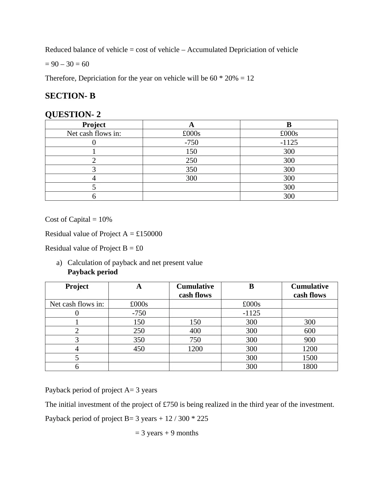
QUESTION- 2
Project A B
Net cash flows in: £000s £000s
0 -750 -1125
1 150 300
2 250 300
3 350 300
4 300 300
5 300
6 300
Cost of Capital = 10%
Residual value of Project A = £150000
Residual value of Project B = £0
a) Calculation of payback and net present value
Payback period
Project A Cumulative
cash flows
B Cumulative
cash flows
Net cash flows in: £000s £000s
0 -750 -1125
1 150 150 300 300
2 250 400 300 600
3 350 750 300 900
4 450 1200 300 1200
5 300 1500
6 300 1800
Payback period of project A= 3 years
The initial investment of the project of £750 is being realized in the third year of the investment.
Payback period of project B= 3 years + 12 / 300 * 225
= 3 years + 9 months
= 90 – 30 = 60
Therefore, Depriciation for the year on vehicle will be 60 * 20% = 12
SECTION- B
QUESTION- 2
Project A B
Net cash flows in: £000s £000s
0 -750 -1125
1 150 300
2 250 300
3 350 300
4 300 300
5 300
6 300
Cost of Capital = 10%
Residual value of Project A = £150000
Residual value of Project B = £0
a) Calculation of payback and net present value
Payback period
Project A Cumulative
cash flows
B Cumulative
cash flows
Net cash flows in: £000s £000s
0 -750 -1125
1 150 150 300 300
2 250 400 300 600
3 350 750 300 900
4 450 1200 300 1200
5 300 1500
6 300 1800
Payback period of project A= 3 years
The initial investment of the project of £750 is being realized in the third year of the investment.
Payback period of project B= 3 years + 12 / 300 * 225
= 3 years + 9 months
= 3 years and 9 months
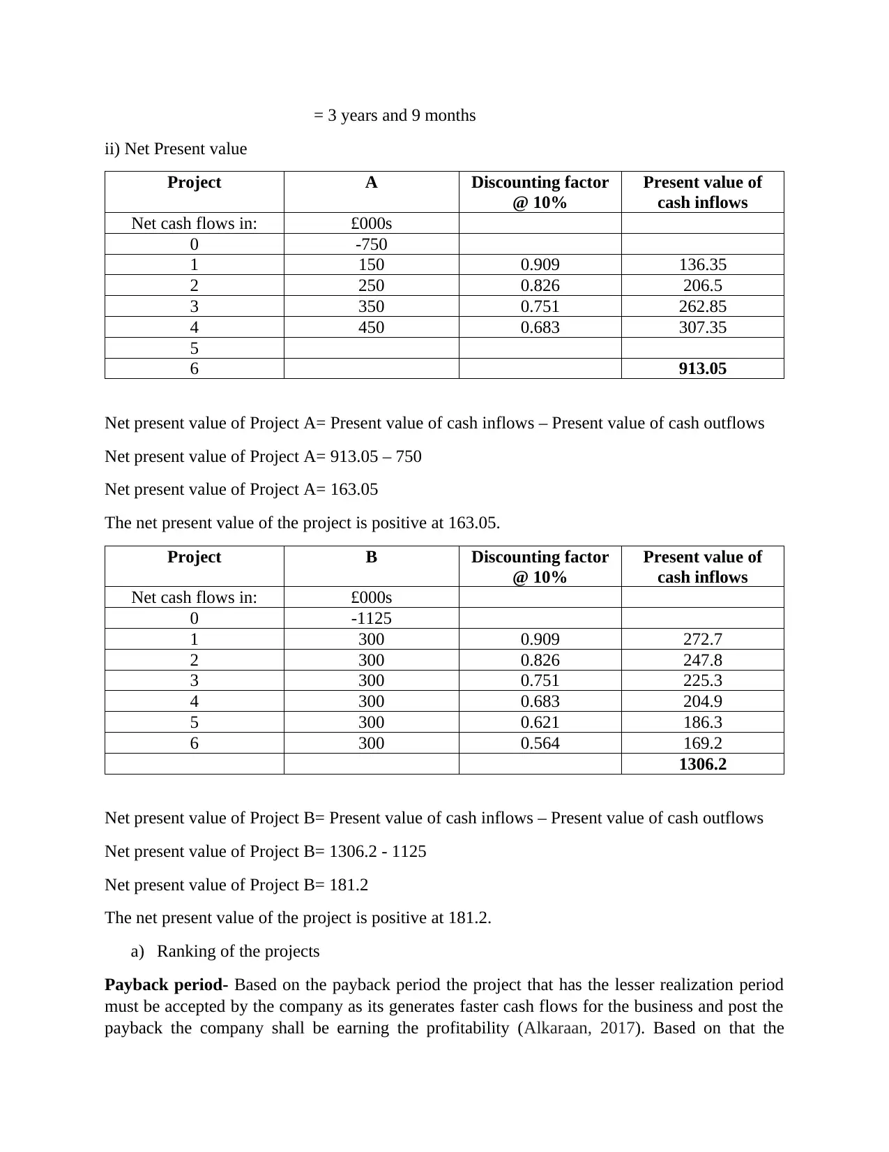
ii) Net Present value
Project A Discounting factor
@ 10%
Present value of
cash inflows
Net cash flows in: £000s
0 -750
1 150 0.909 136.35
2 250 0.826 206.5
3 350 0.751 262.85
4 450 0.683 307.35
5
6 913.05
Net present value of Project A= Present value of cash inflows – Present value of cash outflows
Net present value of Project A= 913.05 – 750
Net present value of Project A= 163.05
The net present value of the project is positive at 163.05.
Project B Discounting factor
@ 10%
Present value of
cash inflows
Net cash flows in: £000s
0 -1125
1 300 0.909 272.7
2 300 0.826 247.8
3 300 0.751 225.3
4 300 0.683 204.9
5 300 0.621 186.3
6 300 0.564 169.2
1306.2
Net present value of Project B= Present value of cash inflows – Present value of cash outflows
Net present value of Project B= 1306.2 - 1125
Net present value of Project B= 181.2
The net present value of the project is positive at 181.2.
a) Ranking of the projects
Payback period- Based on the payback period the project that has the lesser realization period
must be accepted by the company as its generates faster cash flows for the business and post the
payback the company shall be earning the profitability (Alkaraan, 2017). Based on that the
⊘ This is a preview!⊘
Do you want full access?
Subscribe today to unlock all pages.
Trusted by 1+ million students worldwide
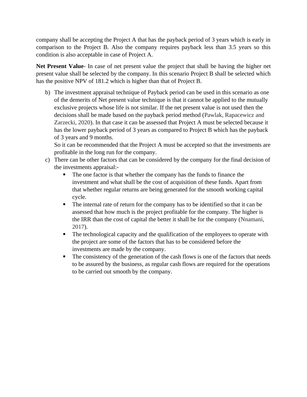
company shall be accepting the Project A that has the payback period of 3 years which is early in
comparison to the Project B. Also the company requires payback less than 3.5 years so this
condition is also acceptable in case of Project A.
Net Present Value- In case of net present value the project that shall be having the higher net
present value shall be selected by the company. In this scenario Project B shall be selected which
has the positive NPV of 181.2 which is higher than that of Project B.
b) The investment appraisal technique of Payback period can be used in this scenario as one
of the demerits of Net present value technique is that it cannot be applied to the mutually
exclusive projects whose life is not similar. If the net present value is not used then the
decisions shall be made based on the payback period method (Pawlak, Rapacewicz and
Zarzecki, 2020). In that case it can be assessed that Project A must be selected because it
has the lower payback period of 3 years as compared to Project B which has the payback
of 3 years and 9 months.
So it can be recommended that the Project A must be accepted so that the investments are
profitable in the long run for the company.
c) There can be other factors that can be considered by the company for the final decision of
the investments appraisal:-
The one factor is that whether the company has the funds to finance the
investment and what shall be the cost of acquisition of these funds. Apart from
that whether regular returns are being generated for the smooth working capital
cycle.
The internal rate of return for the company has to be identified so that it can be
assessed that how much is the project profitable for the company. The higher is
the IRR than the cost of capital the better it shall be for the company (Nnamani,
2017).
The technological capacity and the qualification of the employees to operate with
the project are some of the factors that has to be considered before the
investments are made by the company.
The consistency of the generation of the cash flows is one of the factors that needs
to be assured by the business, as regular cash flows are required for the operations
to be carried out smooth by the company.
Paraphrase This Document
Need a fresh take? Get an instant paraphrase of this document with our AI Paraphraser
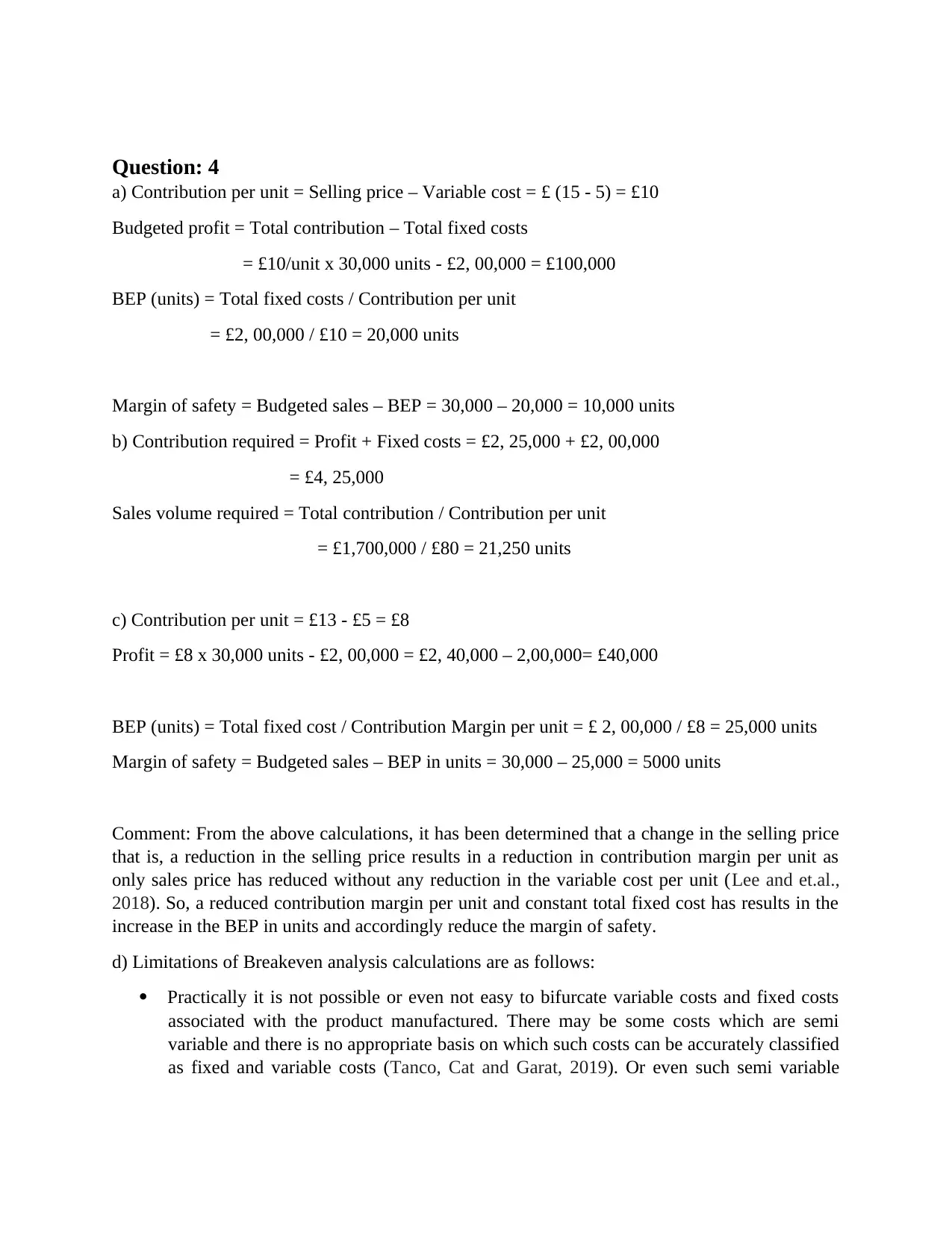
Question: 4
a) Contribution per unit = Selling price – Variable cost = £ (15 - 5) = £10
Budgeted profit = Total contribution – Total fixed costs
= £10/unit x 30,000 units - £2, 00,000 = £100,000
BEP (units) = Total fixed costs / Contribution per unit
= £2, 00,000 / £10 = 20,000 units
Margin of safety = Budgeted sales – BEP = 30,000 – 20,000 = 10,000 units
b) Contribution required = Profit + Fixed costs = £2, 25,000 + £2, 00,000
= £4, 25,000
Sales volume required = Total contribution / Contribution per unit
= £1,700,000 / £80 = 21,250 units
c) Contribution per unit = £13 - £5 = £8
Profit = £8 x 30,000 units - £2, 00,000 = £2, 40,000 – 2,00,000= £40,000
BEP (units) = Total fixed cost / Contribution Margin per unit = £ 2, 00,000 / £8 = 25,000 units
Margin of safety = Budgeted sales – BEP in units = 30,000 – 25,000 = 5000 units
Comment: From the above calculations, it has been determined that a change in the selling price
that is, a reduction in the selling price results in a reduction in contribution margin per unit as
only sales price has reduced without any reduction in the variable cost per unit (Lee and et.al.,
2018). So, a reduced contribution margin per unit and constant total fixed cost has results in the
increase in the BEP in units and accordingly reduce the margin of safety.
d) Limitations of Breakeven analysis calculations are as follows:
Practically it is not possible or even not easy to bifurcate variable costs and fixed costs
associated with the product manufactured. There may be some costs which are semi
variable and there is no appropriate basis on which such costs can be accurately classified
as fixed and variable costs (Tanco, Cat and Garat, 2019). Or even such semi variable
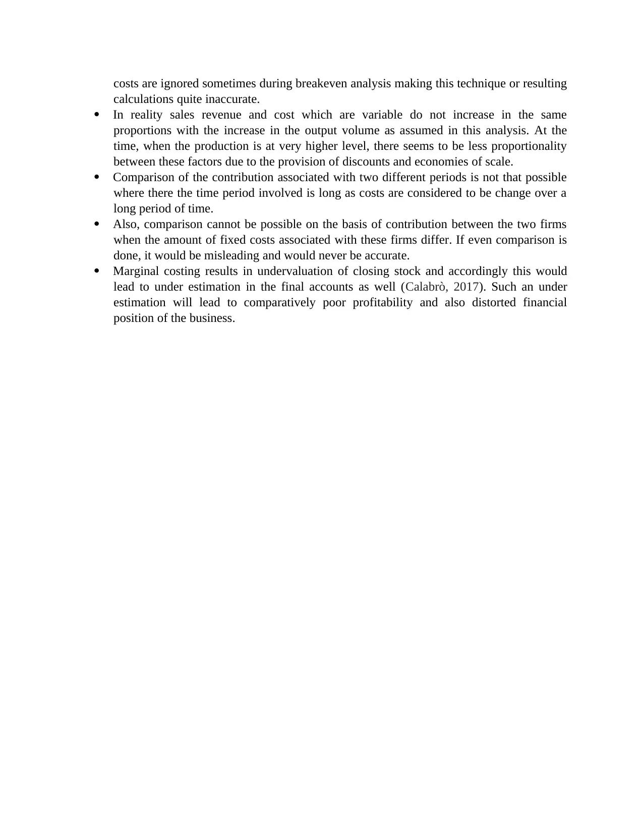
costs are ignored sometimes during breakeven analysis making this technique or resulting
calculations quite inaccurate.
In reality sales revenue and cost which are variable do not increase in the same
proportions with the increase in the output volume as assumed in this analysis. At the
time, when the production is at very higher level, there seems to be less proportionality
between these factors due to the provision of discounts and economies of scale.
Comparison of the contribution associated with two different periods is not that possible
where there the time period involved is long as costs are considered to be change over a
long period of time.
Also, comparison cannot be possible on the basis of contribution between the two firms
when the amount of fixed costs associated with these firms differ. If even comparison is
done, it would be misleading and would never be accurate.
Marginal costing results in undervaluation of closing stock and accordingly this would
lead to under estimation in the final accounts as well (Calabrò, 2017). Such an under
estimation will lead to comparatively poor profitability and also distorted financial
position of the business.
⊘ This is a preview!⊘
Do you want full access?
Subscribe today to unlock all pages.
Trusted by 1+ million students worldwide
REFERENCES
Alkaraan, F., 2017. Strategic investment appraisal: multidisciplinary perspectives. In Advances
in Mergers and Acquisitions. Emerald Publishing Limited.
Pawlak, M., Rapacewicz, A. and Zarzecki, D., 2020. Investment Appraisal Practice in the
Biggest Companies in Poland. European Research Studies. 23(2). pp.137-147.
Nnamani, O. C., 2017. Application of Quantitative Risk Assessment Techniques in Property
Investment Appraisal in Enugu Urban, Nigeria. Journal of Land Management and
Appraisal. 5(1). pp.23-41.
Calabrò, F., 2017, July. Local communities and management of cultural heritage of the inner
areas. An application of break-even analysis. In International Conference on Computational
Science and Its Applications (pp. 516-531). Springer, Cham.
Tanco, M., Cat, L. and Garat, S., 2019. A break-even analysis for battery electric trucks in Latin
America. Journal of Cleaner Production. 228. pp.1354-1367.
Lee, M., and et.al., 2018. A break-even analysis and impact analysis of residential solar
photovoltaic systems considering state solar incentives. Technological and Economic
Development of Economy. 24(2). pp.358-382.
1 out of 10
Related Documents


Your All-in-One AI-Powered Toolkit for Academic Success.
+13062052269
info@desklib.com
Available 24*7 on WhatsApp / Email
![[object Object]](/_next/static/media/star-bottom.7253800d.svg)
Unlock your academic potential
Copyright © 2020–2026 A2Z Services. All Rights Reserved. Developed and managed by ZUCOL.