MOD005704 - Financial Investment Analysis Report: Investment Analysis

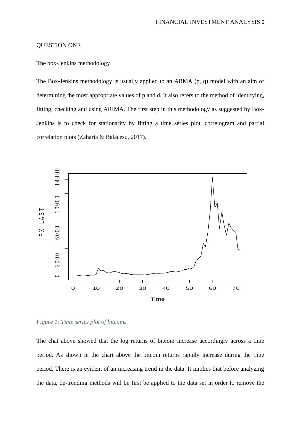
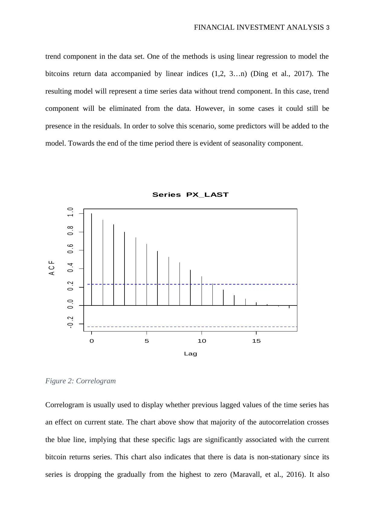
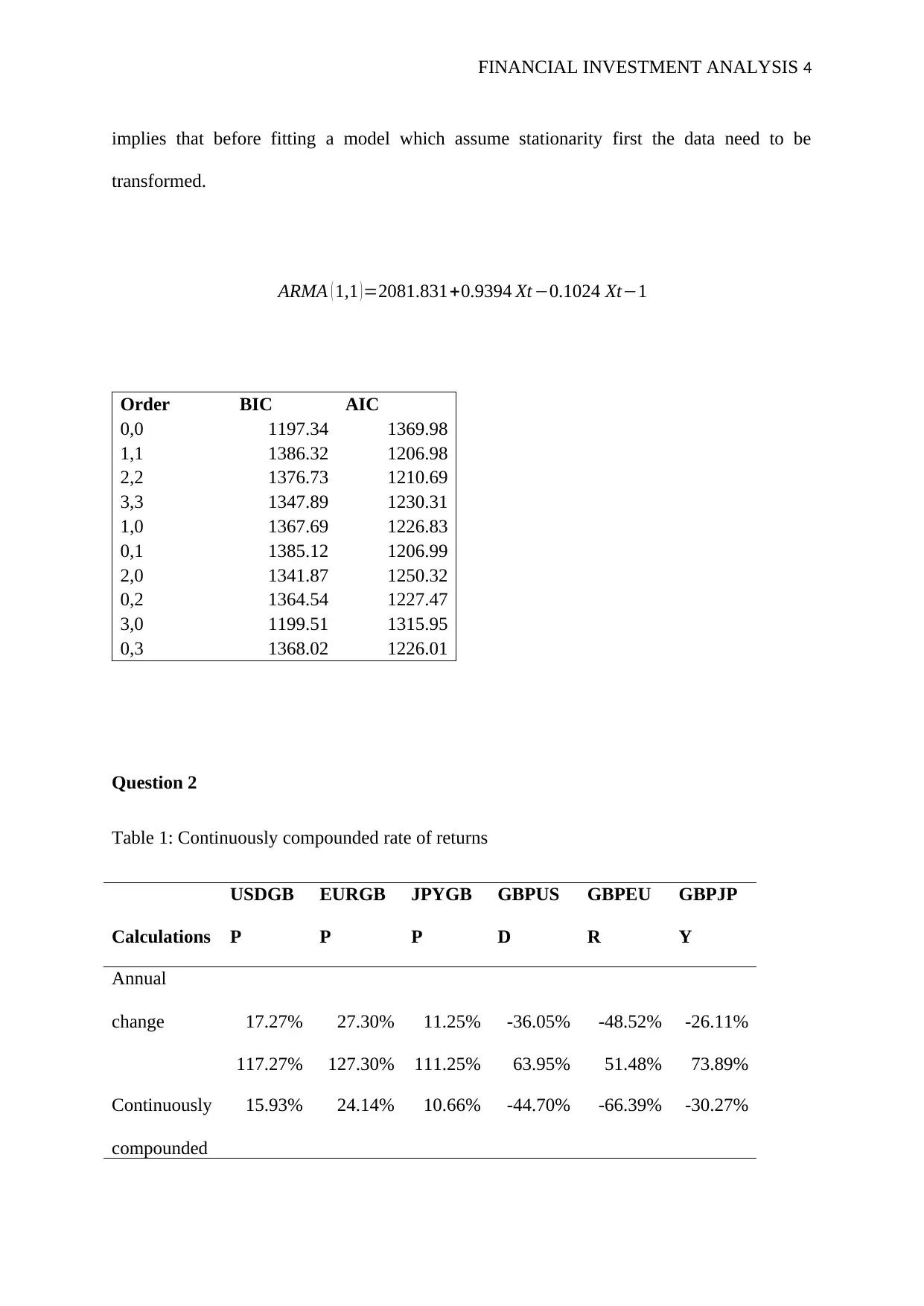
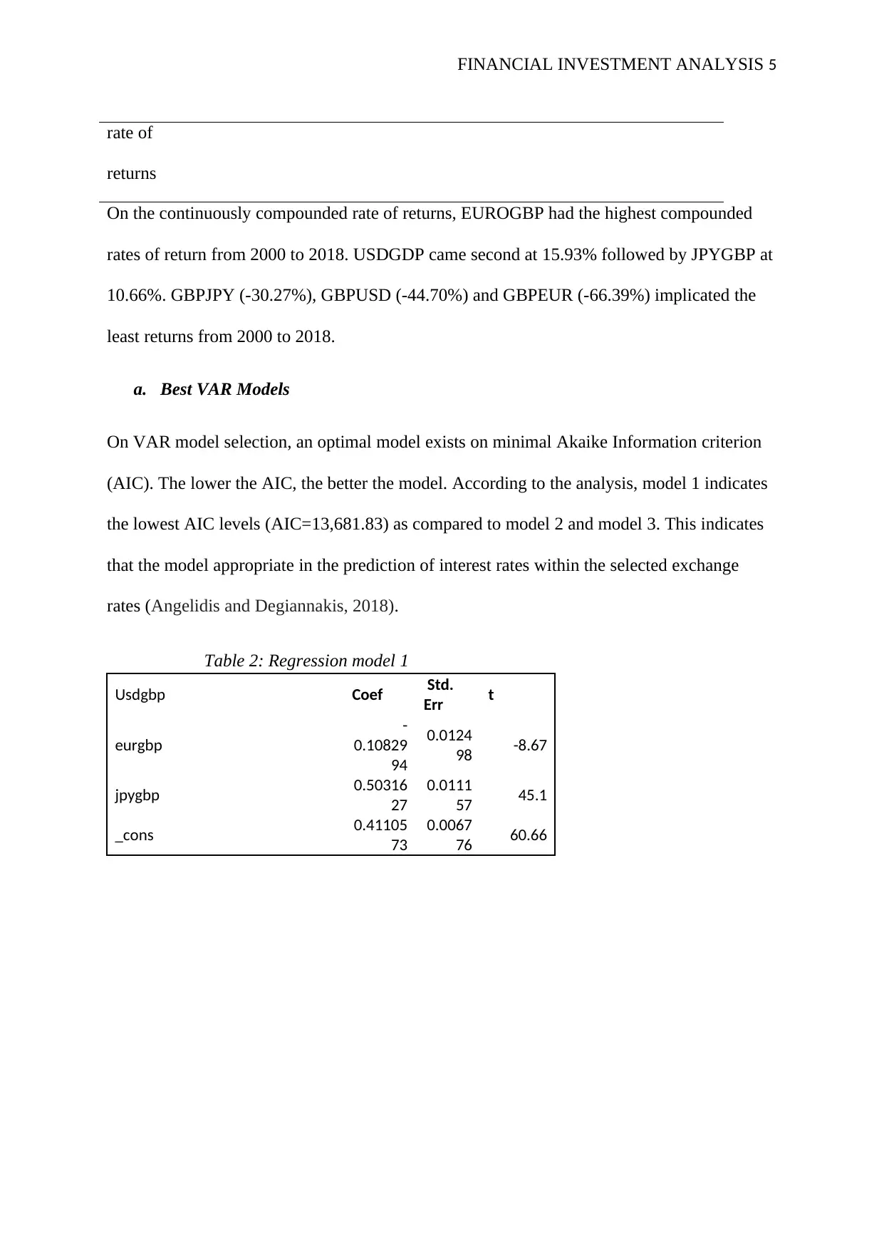
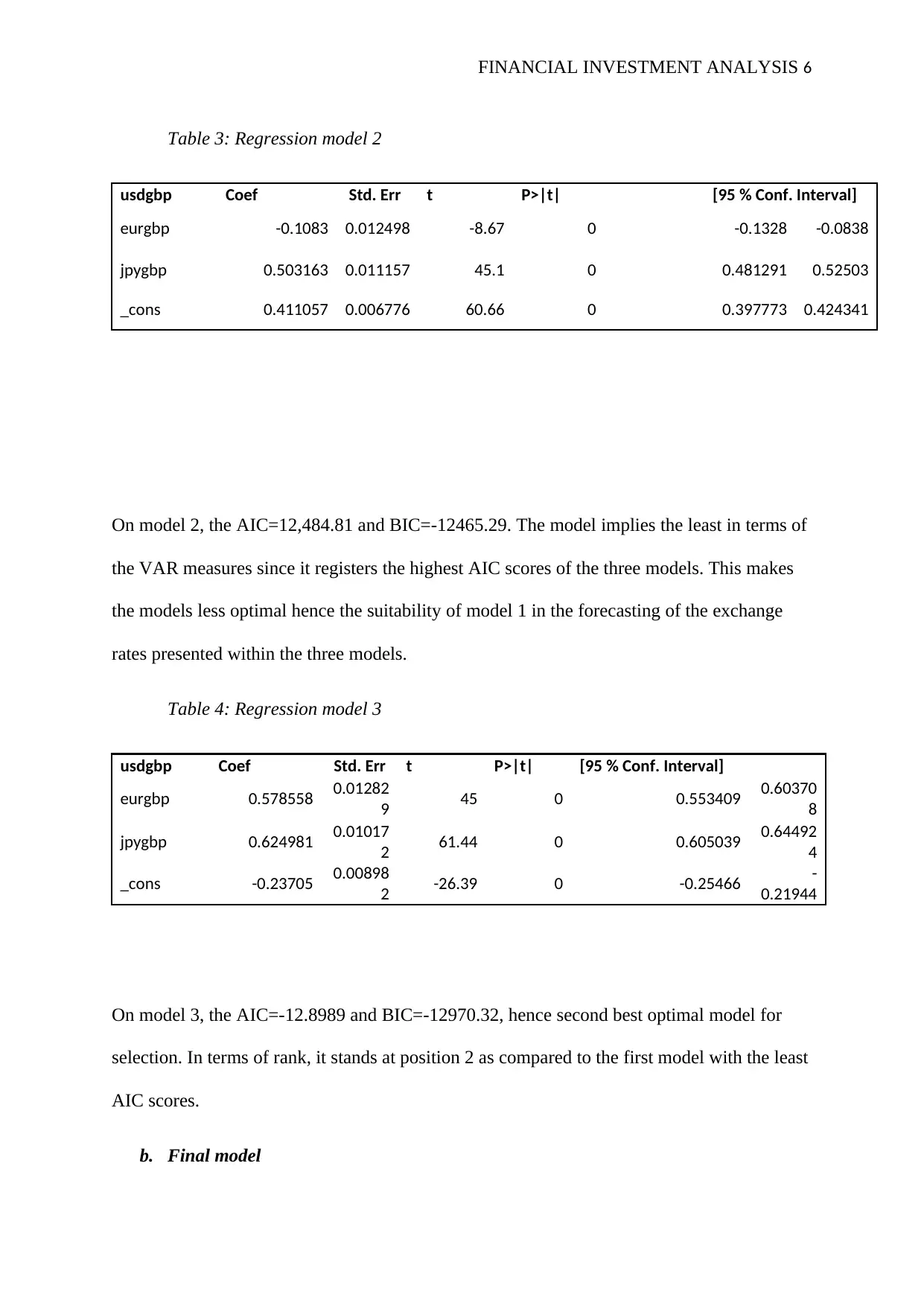
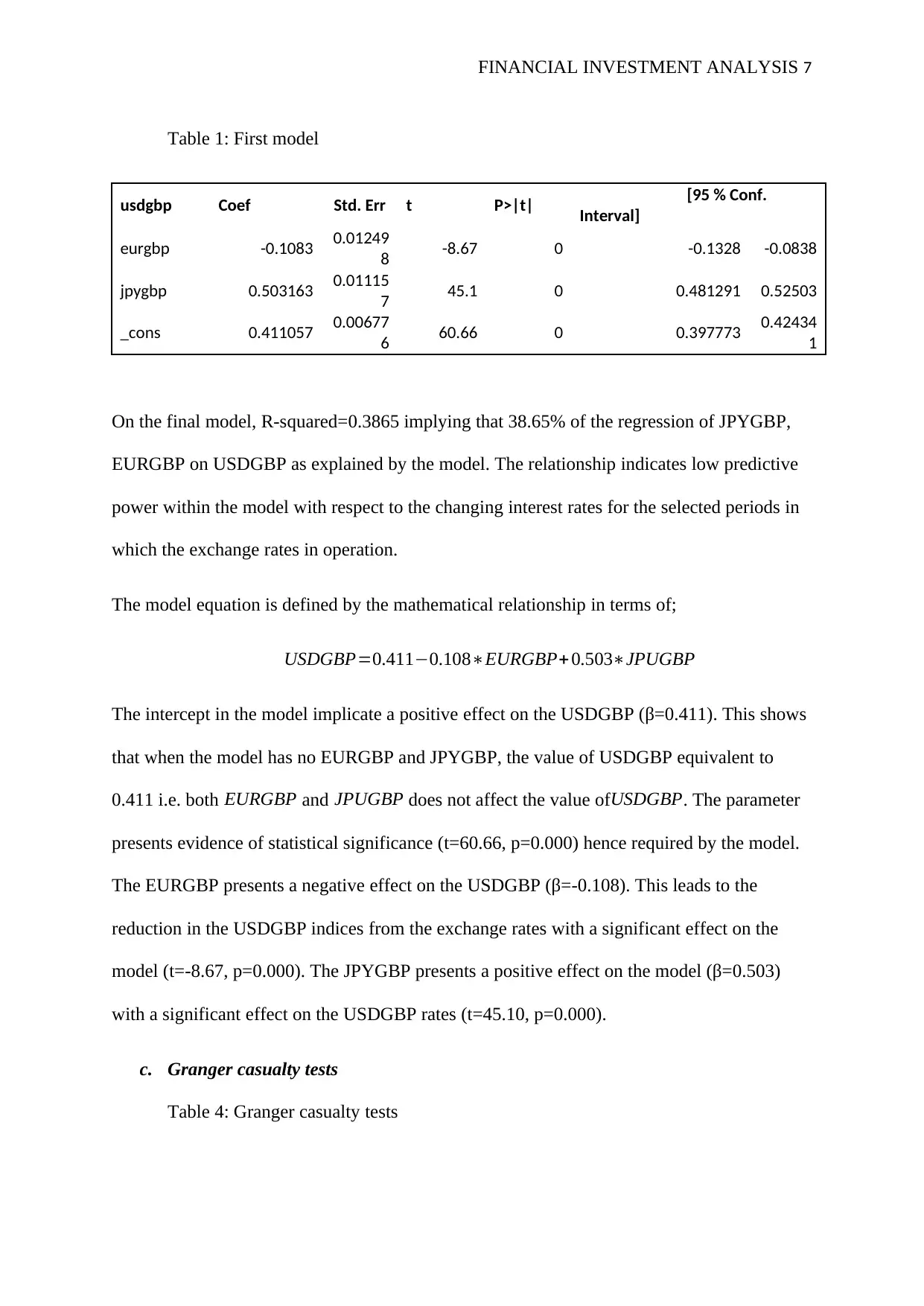
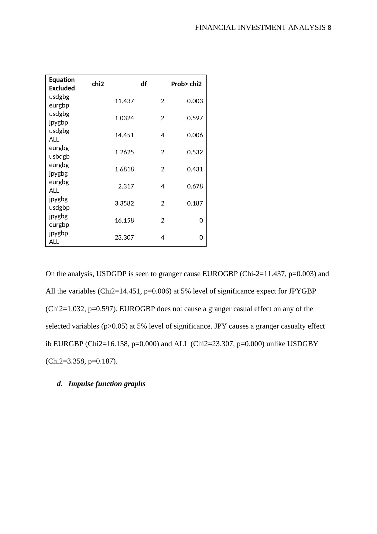
This report provides a financial investment analysis, utilizing the Box-Jenkins methodology to analyze Bitcoin log returns, employing time series plots and correlograms to assess stationarity and autocorrelation. It evaluates continuously compounded rates of return for various currency pairs, identifying EUROGBP as having the highest return from 2000 to 2018. The analysis includes VAR model selection based on the Akaike Information Criterion (AIC), determining that model 1 is the most appropriate for predicting interest rates. Granger causality tests reveal relationships between USDGDP, EUROGBP, and JPYGBP. The report also explores the relationship between future oil prices and spot rates using VAR tests and Engle-Granger 2 step model, concluding with an error correction model and an economic rationale discussing the implications of cointegration or lack thereof on revenue streams and market efficiency. The document is contributed by a student and available on Desklib.

FINANCIAL INVESTMENT ANALYSIS 1
FINANCIAL INVESTMENT ANALYSIS
Course name
Professor’s name
Institution name
City
Date of submission

FINANCIAL INVESTMENT ANALYSIS 2
QUESTION ONE
The box-Jenkins methodology
The Box-Jenkins methodology is usually applied to an ARMA (p, q) model with an aim of
determining the most appropriate values of p and d. It also refers to the method of identifying,
fitting, checking and using ARIMA. The first step in this methodology as suggested by Box-
Jenkins is to check for stationarity by fitting a time series plot, correlogram and partial
correlation plots (Zaharia & Balacesu, 2017).
Time
P X _ L A S T
0 10 20 30 40 50 60 70
0 2 0 0 0 6 0 0 0 1 0 0 0 0 1 4 0 0 0
Figure 1: Time series plot of bitcoins
The chat above showed that the log returns of bitcoin increase accordingly across a time
period. As shown in the chart above the bitcoin returns rapidly increase during the time
period. There is an evident of an increasing trend in the data. It implies that before analyzing
the data, de-trending methods will be first be applied to the data set in order to remove the

FINANCIAL INVESTMENT ANALYSIS 3
trend component in the data set. One of the methods is using linear regression to model the
bitcoins return data accompanied by linear indices (1,2, 3…n) (Ding et al., 2017). The
resulting model will represent a time series data without trend component. In this case, trend
component will be eliminated from the data. However, in some cases it could still be
presence in the residuals. In order to solve this scenario, some predictors will be added to the
model. Towards the end of the time period there is evident of seasonality component.
0 5 10 15
- 0 .2 0 .0 0 .2 0 .4 0 .6 0 .8 1 .0
Lag
A C F
Series PX_LAST
Figure 2: Correlogram
Correlogram is usually used to display whether previous lagged values of the time series has
an effect on current state. The chart above show that majority of the autocorrelation crosses
the blue line, implying that these specific lags are significantly associated with the current
bitcoin returns series. This chart also indicates that there is data is non-stationary since its
series is dropping the gradually from the highest to zero (Maravall, et al., 2016). It also

FINANCIAL INVESTMENT ANALYSIS 4
implies that before fitting a model which assume stationarity first the data need to be
transformed.
ARMA ( 1,1 ) =2081.831+0.9394 Xt −0.1024 Xt−1
Order BIC AIC
0,0 1197.34 1369.98
1,1 1386.32 1206.98
2,2 1376.73 1210.69
3,3 1347.89 1230.31
1,0 1367.69 1226.83
0,1 1385.12 1206.99
2,0 1341.87 1250.32
0,2 1364.54 1227.47
3,0 1199.51 1315.95
0,3 1368.02 1226.01
Question 2
Table 1: Continuously compounded rate of returns
Calculations
USDGB
P
EURGB
P
JPYGB
P
GBPUS
D
GBPEU
R
GBPJP
Y
Annual
change 17.27% 27.30% 11.25% -36.05% -48.52% -26.11%
117.27% 127.30% 111.25% 63.95% 51.48% 73.89%
Continuously
compounded
15.93% 24.14% 10.66% -44.70% -66.39% -30.27%

FINANCIAL INVESTMENT ANALYSIS 5
rate of
returns
On the continuously compounded rate of returns, EUROGBP had the highest compounded
rates of return from 2000 to 2018. USDGDP came second at 15.93% followed by JPYGBP at
10.66%. GBPJPY (-30.27%), GBPUSD (-44.70%) and GBPEUR (-66.39%) implicated the
least returns from 2000 to 2018.
a. Best VAR Models
On VAR model selection, an optimal model exists on minimal Akaike Information criterion
(AIC). The lower the AIC, the better the model. According to the analysis, model 1 indicates
the lowest AIC levels (AIC=13,681.83) as compared to model 2 and model 3. This indicates
that the model appropriate in the prediction of interest rates within the selected exchange
rates (Angelidis and Degiannakis, 2018).
Table 2: Regression model 1
Usdgbp Coef Std.
Err t
eurgbp
-
0.10829
94
0.0124
98 -8.67
jpygbp 0.50316
27
0.0111
57 45.1
_cons 0.41105
73
0.0067
76 60.66

FINANCIAL INVESTMENT ANALYSIS 6
Table 3: Regression model 2
usdgbp Coef Std. Err t P>|t| [95 % Conf. Interval]
eurgbp -0.1083 0.012498 -8.67 0 -0.1328 -0.0838
jpygbp 0.503163 0.011157 45.1 0 0.481291 0.52503
_cons 0.411057 0.006776 60.66 0 0.397773 0.424341
On model 2, the AIC=12,484.81 and BIC=-12465.29. The model implies the least in terms of
the VAR measures since it registers the highest AIC scores of the three models. This makes
the models less optimal hence the suitability of model 1 in the forecasting of the exchange
rates presented within the three models.
Table 4: Regression model 3
usdgbp Coef Std. Err t P>|t| [95 % Conf. Interval]
eurgbp 0.578558 0.01282
9 45 0 0.553409 0.60370
8
jpygbp 0.624981 0.01017
2 61.44 0 0.605039 0.64492
4
_cons -0.23705 0.00898
2 -26.39 0 -0.25466 -
0.21944
On model 3, the AIC=-12.8989 and BIC=-12970.32, hence second best optimal model for
selection. In terms of rank, it stands at position 2 as compared to the first model with the least
AIC scores.
b. Final model

FINANCIAL INVESTMENT ANALYSIS 7
Table 1: First model
usdgbp Coef Std. Err t P>|t| [95 % Conf.
Interval]
eurgbp -0.1083 0.01249
8 -8.67 0 -0.1328 -0.0838
jpygbp 0.503163 0.01115
7 45.1 0 0.481291 0.52503
_cons 0.411057 0.00677
6 60.66 0 0.397773 0.42434
1
On the final model, R-squared=0.3865 implying that 38.65% of the regression of JPYGBP,
EURGBP on USDGBP as explained by the model. The relationship indicates low predictive
power within the model with respect to the changing interest rates for the selected periods in
which the exchange rates in operation.
The model equation is defined by the mathematical relationship in terms of;
USDGBP=0.411−0.108∗EURGBP+0.503∗JPUGBP
The intercept in the model implicate a positive effect on the USDGBP (β=0.411). This shows
that when the model has no EURGBP and JPYGBP, the value of USDGBP equivalent to
0.411 i.e. both EURGBP and JPUGBP does not affect the value ofUSDGBP. The parameter
presents evidence of statistical significance (t=60.66, p=0.000) hence required by the model.
The EURGBP presents a negative effect on the USDGBP (β=-0.108). This leads to the
reduction in the USDGBP indices from the exchange rates with a significant effect on the
model (t=-8.67, p=0.000). The JPYGBP presents a positive effect on the model (β=0.503)
with a significant effect on the USDGBP rates (t=45.10, p=0.000).
c. Granger casualty tests
Table 4: Granger casualty tests

FINANCIAL INVESTMENT ANALYSIS 8
Equation
Excluded chi2 df Prob> chi2
usdgbg
eurgbp 11.437 2 0.003
usdgbg
jpygbp 1.0324 2 0.597
usdgbg
ALL 14.451 4 0.006
eurgbg
usbdgb 1.2625 2 0.532
eurgbg
jpygbg 1.6818 2 0.431
eurgbg
ALL 2.317 4 0.678
jpygbg
usdgbp 3.3582 2 0.187
jpygbg
eurgbp 16.158 2 0
jpygbp
ALL 23.307 4 0
On the analysis, USDGDP is seen to granger cause EUROGBP (Chi-2=11.437, p=0.003) and
All the variables (Chi2=14.451, p=0.006) at 5% level of significance expect for JPYGBP
(Chi2=1.032, p=0.597). EUROGBP does not cause a granger casual effect on any of the
selected variables (p>0.05) at 5% level of significance. JPY causes a granger casualty effect
ib EURGBP (Chi2=16.158, p=0.000) and ALL (Chi2=23.307, p=0.000) unlike USDGBY
(Chi2=3.358, p=0.187).
d. Impulse function graphs

FINANCIAL INVESTMENT ANALYSIS 9
0
.0001
.0002
.0003
0 5 10
order1, eurgbp, usdgbp
95% CI orthogonalized irf
step
Graphs by irfname, impulse variable, and response variable
Figure 1: Impulse function graph of EURGBP and USDGBP
On the graph, the EURGBP and the USDGBP falls between 0.00 and 0.0003, with a constant
levels of significance depicted by the trend.

FINANCIAL INVESTMENT ANALYSIS 10
-.0001
0
.0001
.0002
0 5 10
order1, jpygbp, usdgbp
95% CI orthogonalized irf
step
Graphs by irfname, impulse variable, and response variable
Figure 2: Impulse function graph of JPYGBP and USDGBP
On the graph, the relationship between JPYUSD and USDGBP falls between 0.000 and 0.005
as depicted by the graph. The output shows some constant orthoganized irf at 5% level of
significance (Ronayne, 2011).
Question 3
a. Trend graph
Below is the trend graphical representation

FINANCIAL INVESTMENT ANALYSIS 11
0 50 100 150
0 50 100 150 200 250
time
FUT_PX st
Figure 3: Trend graph of future prices and the spot rates (natural logarithm)
On the graph, the future prices of the oil show changes over time, from a comparatively lower
price to some high price with time. The pattern depicted range from high to low, with a
possibility of continuous fall in prices. The spot rates indicate a unitary effect, with no change
on the horizontal axis.
Table 5: VAR tests for spot rates (natural logarithm) and future prices (natural logarithm)

FINANCIAL INVESTMENT ANALYSIS 12
Coef. Std. Err z P>|z| [95 % Conf. Interval]