STAT6003: Financial Decisions - Multiple Regression Analysis Report
VerifiedAdded on 2023/01/18
|15
|3055
|88
Report
AI Summary
This report presents a comprehensive analysis of financial data using multiple linear regression. The assignment involves developing a multiple linear regression model with one dependent variable (market price) and four independent variables (Sydney price index, annual % change, total number of square meters, and age of house) using Excel. The report includes data plotting, model development, interpretation of coefficients, and assessment of statistical significance, including R-squared and confidence intervals. It compares the full model with a newly estimated model, discussing the relationships between variables and their impact on market price predictions. The analysis aims to aid financial decision-making through the application of statistical techniques.

Running head: STATISTICS FOR FINANCIAL DECISIONS
1
Statistics for Financial Decisions Using Excel
Name of Author
Class Name
Name of School
1
Statistics for Financial Decisions Using Excel
Name of Author
Class Name
Name of School
Paraphrase This Document
Need a fresh take? Get an instant paraphrase of this document with our AI Paraphraser
STATISTICS FOR FINANCIAL DECISIONS 2
Abstract
The requirement of this assignment is the analysis of financial data using excel to help
make appropriate financial decisions. In the process of analysis, a regression model is supposed
to be developed. The regression model by chance is supposed to have one dependent variable
and four independent variables. From the idea of regression models, a model with more than one
independent variable is a multiple linear regression model. Hence what we actually are expected
to have is a multiple linear regression model. The actual model will look something like;
Y = β0 + β1 X1 + β2 X2 + β3 X3 + β4 X4 + ε (Harrell, 2015). Where Y is treated as the value of the
dependent variable, β0 is treated as the regression constant, β1 partial regression coefficients of
the first variable, β2 partial regression coefficient of the second variable, β3 partial regression
coefficient of the third variable, β4 partial regression coefficient of the fourth coefficient and ε is
treated as the error term.
Introduction
In this section of one of them, a statement that we are supposed to do is the rationale of
the model that we have developed via analysis. Our model is a multiple linear regression which
basically has got four independent variables and one dependent variable, unlike simple linear
regression which has one independent variable. Multiple linear regressions, our model, is
basically tracing its foundation from the correlation analysis. The first independent variable, in
analysis, explains the most of variance whereas the second independent variable explains the
second most of the variance and so on. In summary, the independent variables, help in analysis
to explain a proportional percentage of the variance of the dependent variable. Our model
replicates the identification related to important independent variables (Riley, Jackson, Salanti,
STATISTICS FOR FINANCIAL DECISIONS 3
Burke, Price, Kirkham & White, 2017). One disadvantage is that the model replicates error as
well. As it is known though, there is no model that is always perfect in the analysis (Akinwande,
Dikko & Samson, 2015).
The sample size of the model developed is fifteen cases for each predictor. This means
that for each independent variable there are actually fifteen observations. This is evident even
when you look at the multiple linear regression results ( Bretz, Hothorn & Westfall, 2016).
The dependent variable is the market price with a unit measurement of US Dollars,
something that is supposed to be determined by the model. The independent variables are;
Sydney price index, annual % change measured in percentage, the total number of square meters
measured in square meters and age of house measured in years.
Plotting
0 50 100 150 200 250 300 350 400
0
200
400
600
800
1000
1200
Age of house (years) Total number of square meters
Annual % change Sydney price Index Figure 1
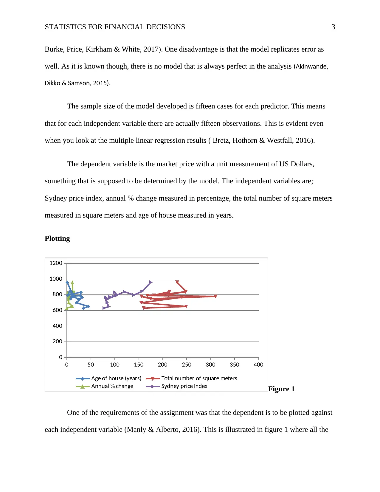
One of the requirements of the assignment was that the dependent is to be plotted against
each independent variable (Manly & Alberto, 2016). This is illustrated in figure 1 where all the
Burke, Price, Kirkham & White, 2017). One disadvantage is that the model replicates error as
well. As it is known though, there is no model that is always perfect in the analysis (Akinwande,
Dikko & Samson, 2015).
The sample size of the model developed is fifteen cases for each predictor. This means
that for each independent variable there are actually fifteen observations. This is evident even
when you look at the multiple linear regression results ( Bretz, Hothorn & Westfall, 2016).
The dependent variable is the market price with a unit measurement of US Dollars,
something that is supposed to be determined by the model. The independent variables are;
Sydney price index, annual % change measured in percentage, the total number of square meters
measured in square meters and age of house measured in years.
Plotting
0 50 100 150 200 250 300 350 400
0
200
400
600
800
1000
1200
Age of house (years) Total number of square meters
Annual % change Sydney price Index Figure 1
One of the requirements of the assignment was that the dependent is to be plotted against
each independent variable (Manly & Alberto, 2016). This is illustrated in figure 1 where all the
⊘ This is a preview!⊘
Do you want full access?
Subscribe today to unlock all pages.
Trusted by 1+ million students worldwide
STATISTICS FOR FINANCIAL DECISIONS 4
plots for the respective variables are made. The variable; the age of house ranges from 0 to a
maximum of 45 hence the clustering to the extreme left. The actual data values when plotted will
produce a curve that crosses itself more than once. The total number of square meters being a
complete larger set of values, you find that the curve is out farther in the graph. It too has
crossing points on itself. Sydney price index keeps on rising, but the percentage change rises and
drops with it being at the extreme left as the changes are minimal but also produces a curve that
crosses itself (Mirman, 2017).
Full Model
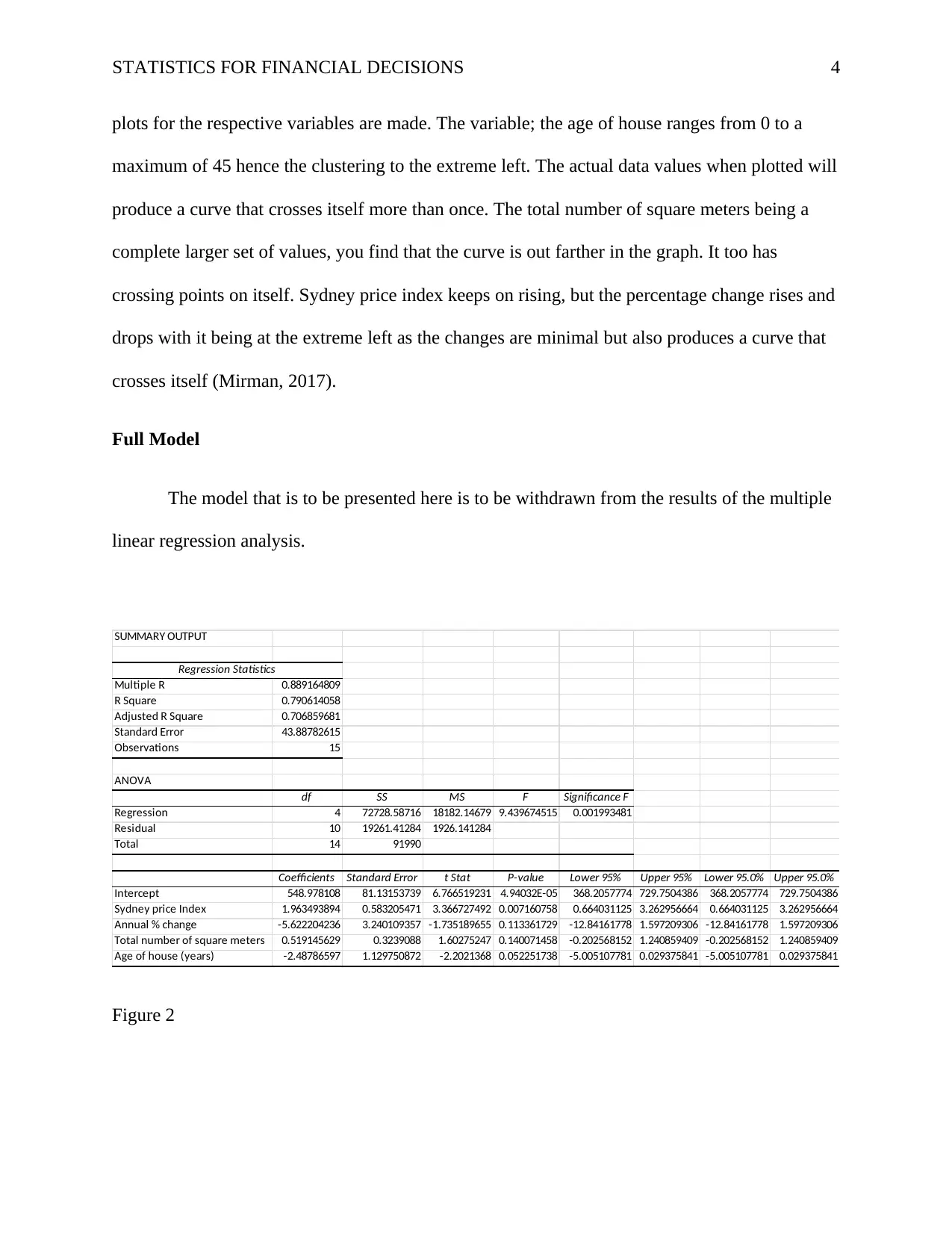
The model that is to be presented here is to be withdrawn from the results of the multiple
linear regression analysis.
SUMMARY OUTPUT
Regression Statistics
Multiple R 0.889164809
R Square 0.790614058
Adjusted R Square 0.706859681
Standard Error 43.88782615
Observations 15
ANOVA
df SS MS F Significance F
Regression 4 72728.58716 18182.14679 9.439674515 0.001993481
Residual 10 19261.41284 1926.141284
Total 14 91990
Coefficients Standard Error t Stat P-value Lower 95% Upper 95% Lower 95.0% Upper 95.0%
Intercept 548.978108 81.13153739 6.766519231 4.94032E-05 368.2057774 729.7504386 368.2057774 729.7504386
Sydney price Index 1.963493894 0.583205471 3.366727492 0.007160758 0.664031125 3.262956664 0.664031125 3.262956664
Annual % change -5.622204236 3.240109357 -1.735189655 0.113361729 -12.84161778 1.597209306 -12.84161778 1.597209306
Total number of square meters 0.519145629 0.3239088 1.60275247 0.140071458 -0.202568152 1.240859409 -0.202568152 1.240859409
Age of house (years) -2.48786597 1.129750872 -2.2021368 0.052251738 -5.005107781 0.029375841 -5.005107781 0.029375841
Figure 2
plots for the respective variables are made. The variable; the age of house ranges from 0 to a
maximum of 45 hence the clustering to the extreme left. The actual data values when plotted will
produce a curve that crosses itself more than once. The total number of square meters being a
complete larger set of values, you find that the curve is out farther in the graph. It too has
crossing points on itself. Sydney price index keeps on rising, but the percentage change rises and
drops with it being at the extreme left as the changes are minimal but also produces a curve that
crosses itself (Mirman, 2017).
Full Model
The model that is to be presented here is to be withdrawn from the results of the multiple
linear regression analysis.
SUMMARY OUTPUT
Regression Statistics
Multiple R 0.889164809
R Square 0.790614058
Adjusted R Square 0.706859681
Standard Error 43.88782615
Observations 15
ANOVA
df SS MS F Significance F
Regression 4 72728.58716 18182.14679 9.439674515 0.001993481
Residual 10 19261.41284 1926.141284
Total 14 91990
Coefficients Standard Error t Stat P-value Lower 95% Upper 95% Lower 95.0% Upper 95.0%
Intercept 548.978108 81.13153739 6.766519231 4.94032E-05 368.2057774 729.7504386 368.2057774 729.7504386
Sydney price Index 1.963493894 0.583205471 3.366727492 0.007160758 0.664031125 3.262956664 0.664031125 3.262956664
Annual % change -5.622204236 3.240109357 -1.735189655 0.113361729 -12.84161778 1.597209306 -12.84161778 1.597209306
Total number of square meters 0.519145629 0.3239088 1.60275247 0.140071458 -0.202568152 1.240859409 -0.202568152 1.240859409
Age of house (years) -2.48786597 1.129750872 -2.2021368 0.052251738 -5.005107781 0.029375841 -5.005107781 0.029375841
Figure 2
Paraphrase This Document
Need a fresh take? Get an instant paraphrase of this document with our AI Paraphraser
STATISTICS FOR FINANCIAL DECISIONS 5
Going by the requirement of the question to this section we will follow the model of the
representative model that we had written in the abstract section but this time we will include the
coefficients with the intercept being β0 and the Sydney price index representing β1, a partial
regression coefficient and so on. Therefore our actual model for the assignment will be;
Y = 548.98 + 1.96X1 -5.62X2 + 0.52X3 -2.49X4 + ε. As you can see the coefficients and the
intercept are all drawn from the coefficient column of the results of the regression model
analysis. X1 is Sydney price index, X2 annual % change, X3 is the total number of square meters,
X4 is an age of a house in years and Y is the market price (Faraway, 2016).
Least Squares Regression Model
Least squares regression model too just like multiple linear regressions was founded on
correlation analysis. Only that it has one and only one independent variable. By this we get the
model; Y = β0 + β1 X1 + ε. β0 is the intercept parameter and β1 is the slope parameter. ε is the error
term. Y is the predicted value (Carroll, 2017).
Estimated coefficients and significant values
In this section, we will interpret the estimated coefficients and discuss their significant
values. Before doing anything, we must inspect the p-values that correspond to the coefficients
of our independent variables. The p-value that is 0.05 or greater is going to be excluded. This
value shows that the predictive value that corresponds to that particular independent variable is
not of significance in predicting our outcomes. From the values of the table, the only p-values
values that are equal to 0.05 or over are those that correspond to annual % change and the total
number of square meters. Only these are statistically insignificant whereas the rest are. It is
STATISTICS FOR FINANCIAL DECISIONS 6
advisable to drop the respective variables in order to rerun the model for better results (Wood,
2017).
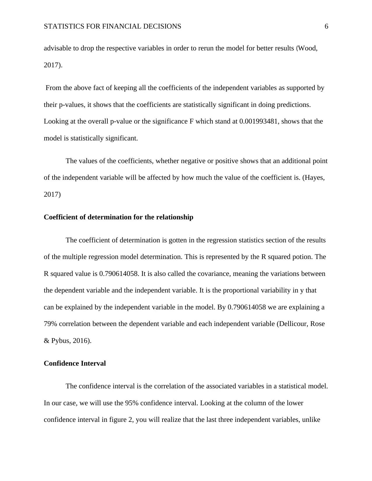
From the above fact of keeping all the coefficients of the independent variables as supported by
their p-values, it shows that the coefficients are statistically significant in doing predictions.
Looking at the overall p-value or the significance F which stand at 0.001993481, shows that the
model is statistically significant.
The values of the coefficients, whether negative or positive shows that an additional point
of the independent variable will be affected by how much the value of the coefficient is. (Hayes,
2017)
Coefficient of determination for the relationship
The coefficient of determination is gotten in the regression statistics section of the results
of the multiple regression model determination. This is represented by the R squared potion. The
R squared value is 0.790614058. It is also called the covariance, meaning the variations between
the dependent variable and the independent variable. It is the proportional variability in y that
can be explained by the independent variable in the model. By 0.790614058 we are explaining a
79% correlation between the dependent variable and each independent variable (Dellicour, Rose
& Pybus, 2016).
Confidence Interval
The confidence interval is the correlation of the associated variables in a statistical model.
In our case, we will use the 95% confidence interval. Looking at the column of the lower
confidence interval in figure 2, you will realize that the last three independent variables, unlike
advisable to drop the respective variables in order to rerun the model for better results (Wood,
2017).
From the above fact of keeping all the coefficients of the independent variables as supported by
their p-values, it shows that the coefficients are statistically significant in doing predictions.
Looking at the overall p-value or the significance F which stand at 0.001993481, shows that the
model is statistically significant.
The values of the coefficients, whether negative or positive shows that an additional point
of the independent variable will be affected by how much the value of the coefficient is. (Hayes,
2017)
Coefficient of determination for the relationship
The coefficient of determination is gotten in the regression statistics section of the results
of the multiple regression model determination. This is represented by the R squared potion. The
R squared value is 0.790614058. It is also called the covariance, meaning the variations between
the dependent variable and the independent variable. It is the proportional variability in y that
can be explained by the independent variable in the model. By 0.790614058 we are explaining a
79% correlation between the dependent variable and each independent variable (Dellicour, Rose
& Pybus, 2016).
Confidence Interval
The confidence interval is the correlation of the associated variables in a statistical model.
In our case, we will use the 95% confidence interval. Looking at the column of the lower
confidence interval in figure 2, you will realize that the last three independent variables, unlike
⊘ This is a preview!⊘
Do you want full access?
Subscribe today to unlock all pages.
Trusted by 1+ million students worldwide

STATISTICS FOR FINANCIAL DECISIONS 7
the first independent variable, have got negative values associated with them. This definitely
shows that the actual correlation relation that the respective independent variables with negative
values have with the dependent variable is actually negative. That of the other independent
variable is actually posing a positive correlation.
Moving to the other upper confidence interval you will realize that all the values that are
there are all positive values. This shows that on the upper side the correlation is actually positive
all through for all the independent variables.
The value of 0 in the confidence interval shows that there is no correlation at all. But in our
interval values of the confidence interval, there is no such value in the confidence interval range.
This shows that there lacks no un-correlation. ( Farinotti, Longuevergne, Moholdt, Duethmann,
Mölg, Bolch & Güntner, 2015).
Relationship between the market price and the land size
As per the newly estimated model, the actual relationship between the market price and
the land size in total square meters is that the land size is correlated to the market price 9.8% of
the time. This is shown in the R squared value. For every additional unit of a square meter, the
market price will be an additional of 0.563603274 of the market price that was initially allocated
to the initial square meter value. The standard error, which is the variability of the actual y-
values from the predicted y-values, stands at 0.473897199. This shows that the actual error made
while predicting the market price is 47%. Moving to the p-value, which is the significant value
corresponding to each variable. The p-value of each and every independent variable should be
less than or equal to 5% or 0.05. Looking at the total number of square meters, the p-value is
greater than 0.05 and is standing at 0.25. From the 0.25 p-value, this shows that the independent
Paraphrase This Document
Need a fresh take? Get an instant paraphrase of this document with our AI Paraphraser
STATISTICS FOR FINANCIAL DECISIONS 8
variable is not statistically significant for analysis and therefore should be dropped to pick
another variable to be used in the running of the model. The two variables correlate negatively to
the lower side but positively to the upper side (Skoog, Holler & Crouch 2017).
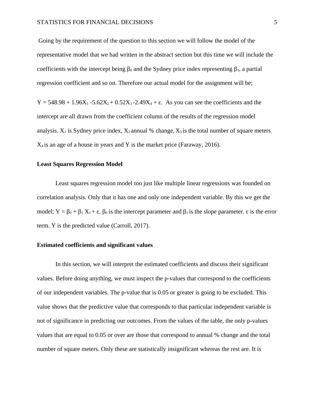
The actual graph as shown below in figure 3, shows multiple crosses of the points. This shows
different areas were sold during different financial, hence the crosses at different points of the
curve (Yandell, 2017).
0 2 4 6 8 10 12
0
2
4
6
8
10
12
Total number of square meters
Total number of square
meters
Estimated Model against the New Model
I comparing the newly estimated model to the old model, using the coefficient of
determination which is the R squared we will realize that the old model is a better model to use
in the correlation process for the business decision because the independent variable dataset, that
is the total number of square meters is correlated to the dependent variable more of the time and
at 79% that the newly estimated model where the correlation between the said independent
variable and the dependent variable stands at 9.8% of the time. In the new model, it is evident to
see that it is less important to use the total number of square meters to determine the market
variable is not statistically significant for analysis and therefore should be dropped to pick
another variable to be used in the running of the model. The two variables correlate negatively to
the lower side but positively to the upper side (Skoog, Holler & Crouch 2017).
The actual graph as shown below in figure 3, shows multiple crosses of the points. This shows
different areas were sold during different financial, hence the crosses at different points of the
curve (Yandell, 2017).
0 2 4 6 8 10 12
0
2
4
6
8
10
12
Total number of square meters
Total number of square
meters
Estimated Model against the New Model
I comparing the newly estimated model to the old model, using the coefficient of
determination which is the R squared we will realize that the old model is a better model to use
in the correlation process for the business decision because the independent variable dataset, that
is the total number of square meters is correlated to the dependent variable more of the time and
at 79% that the newly estimated model where the correlation between the said independent
variable and the dependent variable stands at 9.8% of the time. In the new model, it is evident to
see that it is less important to use the total number of square meters to determine the market

STATISTICS FOR FINANCIAL DECISIONS 9
price. For the old model, it is advisable to use the said independent variable as this would
definitely bring forth.
The standard error of the correlation of the independent and the dependent variables increases
when you use from the old model to the estimated model. Hence the old model is statistically
significant in making estimations. This is because when using the old model, the minimal error
will be encountered as compared to when using the newly estimated model.
The p-value or the significance F for the overall model for the new model stands at
0.2555933 which is more than 0.05, yet that of the old model stands at 0.001993481 which is
less than 0.05. Hence by convention, it is very easy to see that the old model is statistically
significant as opposed to the new estimated model.
From the conclusion, the newly estimated model is the least square regression model. This by
evidence is proven to be less efficient as compared to the multiple linear regressions. Even
though there is no model that is in all averagely statistically perfect but comparing the two, one
surely stands out to be better than the other (Danish, 2016).
Predicting Market Price of a House of 400 Square Meters
Here we will use the least square regression model that we have estimated. The model
system is; Y = β0 + β1 X1 + ε which is actually accorded Y= 659.144 + 0.5636 X1 + 0.4739. The
value of X1 which is the total number of square meters of the house is 400. Replacing 400 in the
equation gives; Y= 659.144 + 0.5636(400) + 0.4739, which then equals 1,885.0579. Since the
value was measured in thousand US dollars the actual value will be $ 1,885,058 (Little & Rubin,
2019).
⊘ This is a preview!⊘
Do you want full access?
Subscribe today to unlock all pages.
Trusted by 1+ million students worldwide
STATISTICS FOR FINANCIAL DECISIONS 10
Conclusion
From the above analysis, it is very evident to see that the actual model that would best fit
regression analysis is the multiple regression model. Given a chance to advise, if there were
several variables, instead of using the least square regression model it is advisable to use multiple
regression model as it gives the best statistical results and it is more statistically significant. The
overall p-value for both cases shows that the real value that is associated to the re-estimated
model is less statistically significant as the value is totally more than the significant value that
stands at 5% or is 0.05.
Paraphrase This Document
Need a fresh take? Get an instant paraphrase of this document with our AI Paraphraser
STATISTICS FOR FINANCIAL DECISIONS 11
References
Akinwande, M. O., Dikko, H. G., & Samson, A. (2015). Variance inflation factor: as a condition
for the inclusion of suppressor variable (s) in regression analysis. Open Journal of
Statistics, 5(07), 754.
Bretz, F., Hothorn, T., & Westfall, P. (2016). Multiple comparisons using R. Chapman and
Hall/CRC.
Carroll, R. J. (2017). Transformation and weighting in regression. Routledge.
Danish, N. P. S. Z. M. (2016). Support vector regression model for predicting the. Bioresour.
Technol, 96, 1292-1296.
Dellicour, S., Rose, R., & Pybus, O. G. (2016). Explaining the geographic spread of emerging
epidemics: a framework for comparing viral phylogenies and environmental landscape
data. BMC Bioinformatics, 17(1), 82.
Faraway, J. J. (2016). Linear models with R. Chapman and Hall/CRC.
Farinotti, D., Longuevergne, L., Moholdt, G., Duethmann, D., Mölg, T., Bolch, T., ... & Güntner,
A. (2015). Substantial glacier mass loss in the Tien Shan over the past 50 years. Nature
Geoscience, 8(9), 716.
Harrell Jr, F. E. (2015). Regression modelling strategies: with applications to linear models,
logistic and ordinal regression, and survival analysis. Springer.
Hayes, A. F. (2017). Introduction to mediation, moderation, and conditional process analysis: A
regression-based approach. Guilford Publications.
STATISTICS FOR FINANCIAL DECISIONS 12
Little, R. J., & Rubin, D. B. (2019). Statistical analysis with missing data (Vol. 793). Wiley.
Manly, B. F., & Alberto, J. A. N. (2016). Multivariate statistical methods: a primer. Chapman
and Hall/CRC.
Mirman, D. (2017). Growth curve analysis and visualization using R. Chapman and Hall/CRC.
Riley, R. D., Jackson, D., Salanti, G., Burke, D. L., Price, M., Kirkham, J., & White, I. R. (2017).
Multivariate and network meta-analysis of multiple outcomes and multiple treatments:
rationale, concepts, and examples. BMJ, 358, j3932.
Skoog, D. A., Holler, F. J., & Crouch, S. R. (2017). Principles of instrumental analysis. Cengage
Learning.
Wood, S. N. (2017). Generalized additive models: an introduction with R. Chapman and
Hall/CRC.
Yandell, B. (2017). Practical data analysis for designed experiments. Routledge.
⊘ This is a preview!⊘
Do you want full access?
Subscribe today to unlock all pages.
Trusted by 1+ million students worldwide
1 out of 15
Related Documents


Your All-in-One AI-Powered Toolkit for Academic Success.
+13062052269
info@desklib.com
Available 24*7 on WhatsApp / Email
![[object Object]](/_next/static/media/star-bottom.7253800d.svg)
Unlock your academic potential
Copyright © 2020–2026 A2Z Services. All Rights Reserved. Developed and managed by ZUCOL.