Analysis of Sales Data Using Regression Techniques

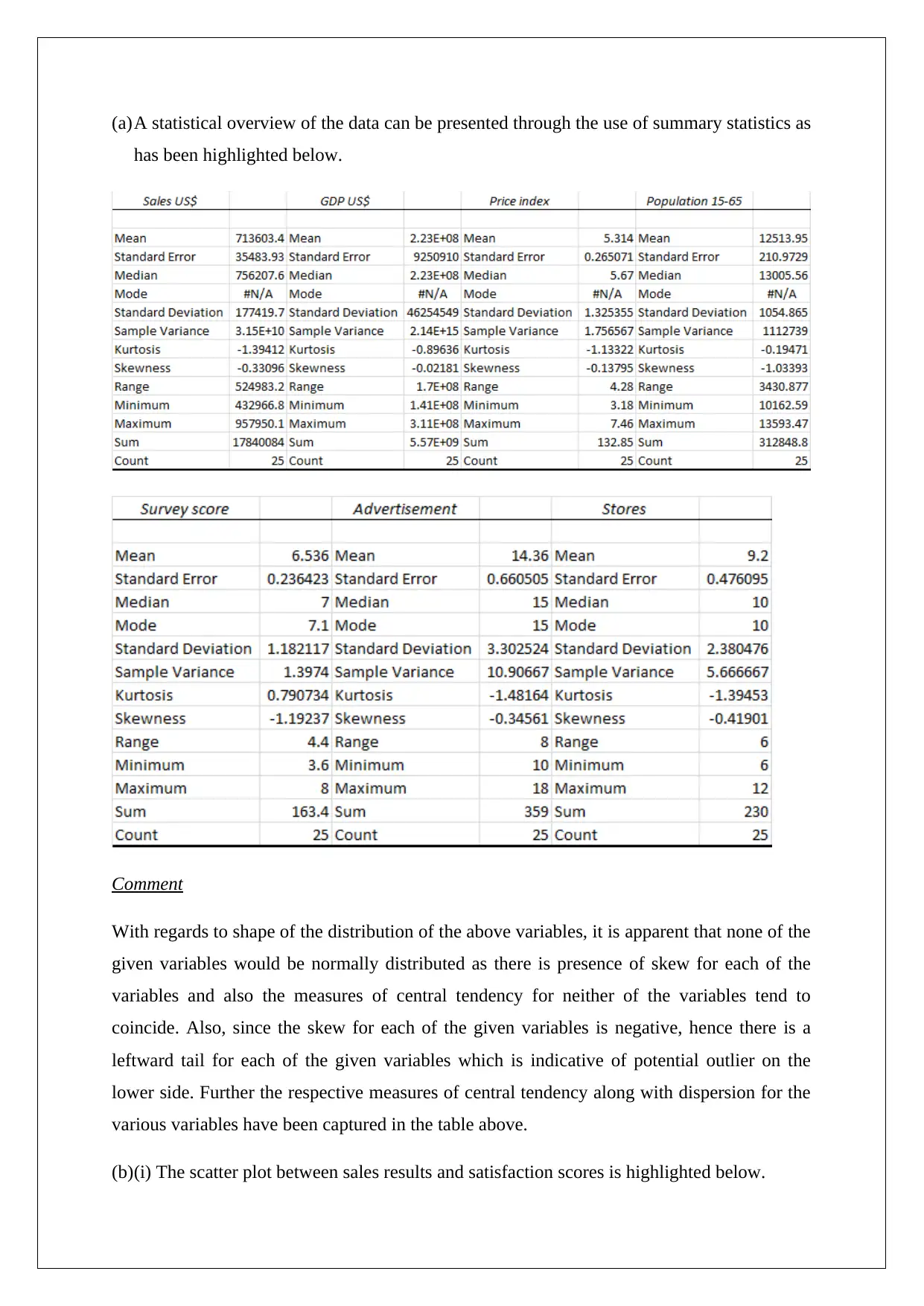
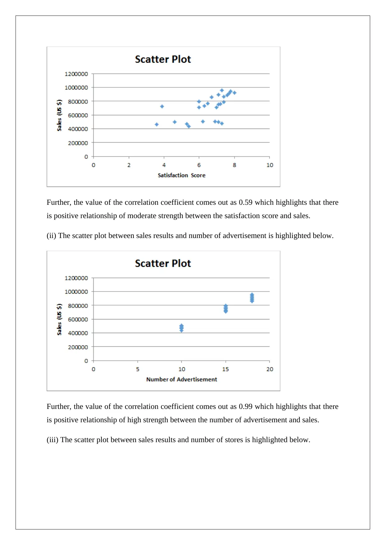
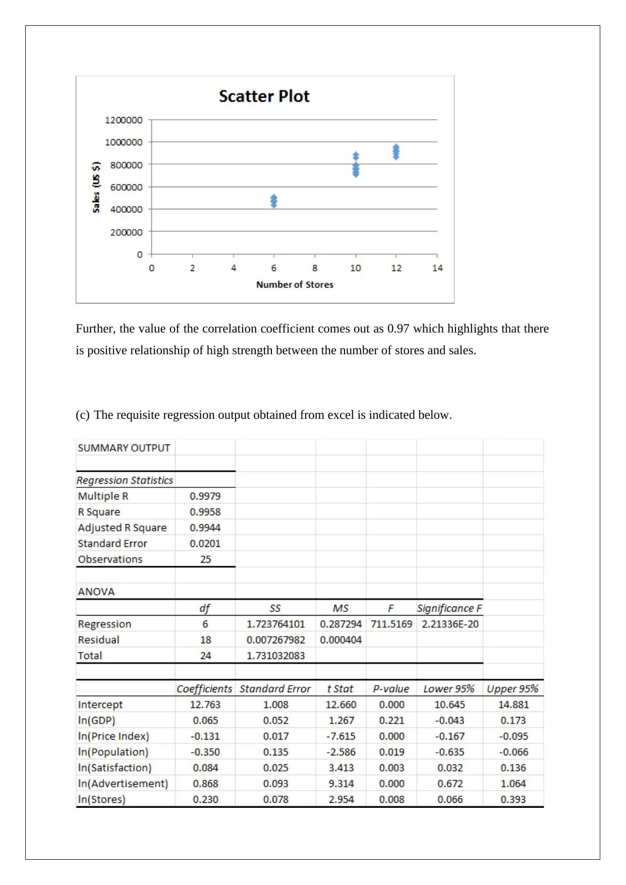
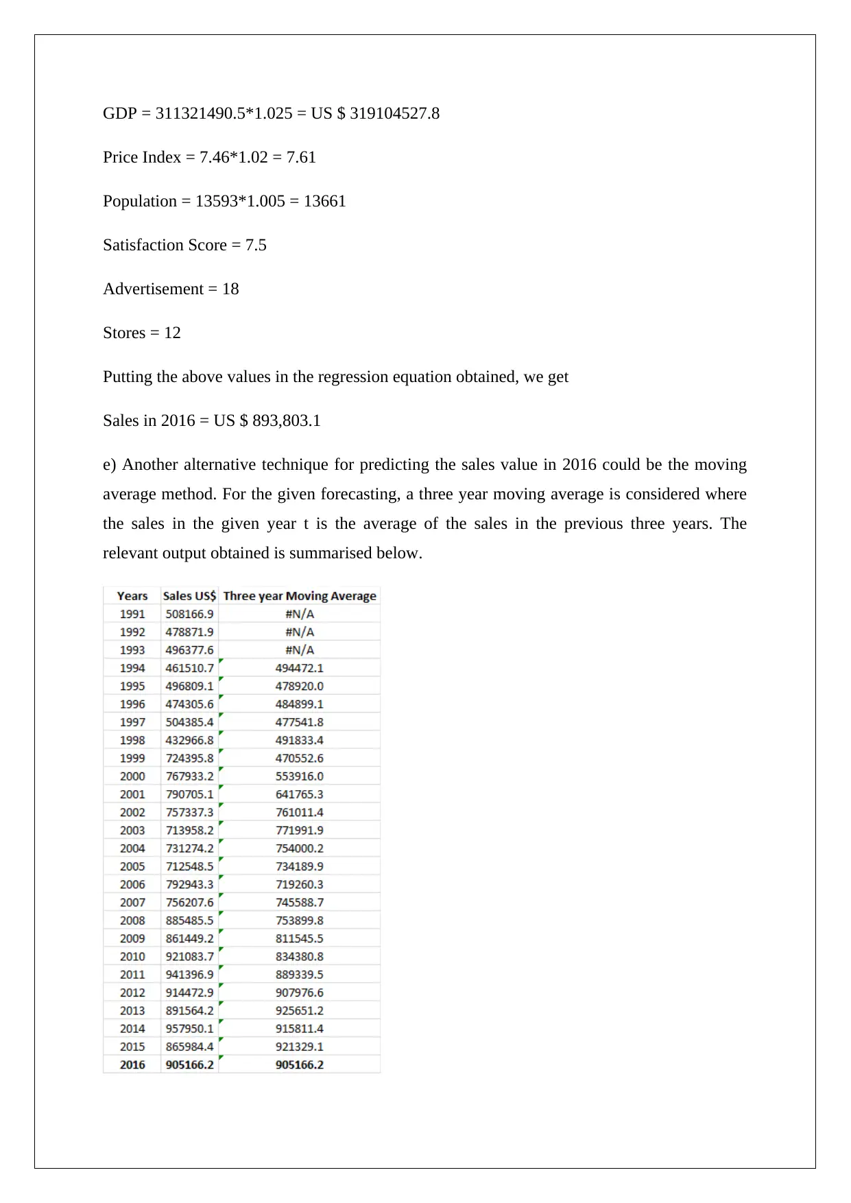
The assignment presents a comprehensive analysis of sales data through the use of descriptive statistics, correlation analysis, regression modeling, and alternative forecasting techniques. Initially, summary statistics are used to characterize the distribution and central tendencies of the dataset variables. The shape of these distributions is assessed for skewness and potential outliers. Scatter plots are employed to visualize relationships between sales results and other factors such as satisfaction scores, advertisement expenditure, and number of stores, revealing varying degrees of correlation strength from moderate to high. A regression model is then formulated using economic indicators such as GDP, Price Index, Population demographics, Satisfaction Score, Advertisement spending, and Number of Stores, providing insights into the variables significantly affecting sales. The statistical significance of the model is affirmed through an ANOVA test with a highly significant F-value, while the coefficient of determination indicates robust explanatory power. Individual regression coefficients are interpreted to quantify the impact of each predictor on sales growth or decline. A forecast for 2016 sales is calculated using both the regression equation and the moving average method, demonstrating alternative predictive approaches within financial decision-making contexts.

STATISTICS FOR FINANCIAL DECISIONS
STUDENT ID:
[Pick the date]

(a)A statistical overview of the data can be presented through the use of summary statistics as
has been highlighted below.
Comment
With regards to shape of the distribution of the above variables, it is apparent that none of the
given variables would be normally distributed as there is presence of skew for each of the
variables and also the measures of central tendency for neither of the variables tend to
coincide. Also, since the skew for each of the given variables is negative, hence there is a
leftward tail for each of the given variables which is indicative of potential outlier on the
lower side. Further the respective measures of central tendency along with dispersion for the
various variables have been captured in the table above.
(b)(i) The scatter plot between sales results and satisfaction scores is highlighted below.

Further, the value of the correlation coefficient comes out as 0.59 which highlights that there
is positive relationship of moderate strength between the satisfaction score and sales.
(ii) The scatter plot between sales results and number of advertisement is highlighted below.
Further, the value of the correlation coefficient comes out as 0.99 which highlights that there
is positive relationship of high strength between the number of advertisement and sales.
(iii) The scatter plot between sales results and number of stores is highlighted below.

Further, the value of the correlation coefficient comes out as 0.97 which highlights that there
is positive relationship of high strength between the number of stores and sales.
(c) The requisite regression output obtained from excel is indicated below.

The requisite regression equation is as states below.
Ln(Sales)=12.763 + 0.065ln(GDP) - 0.131ln(PriceIndex) - 0.350ln(Population) +
0.084ln(Satisfaction) + 0.868ln(Advertisement) + 0.230ln(Stores) + 0.02
Significance of Slope
Hypothesis testing can be done using the t statistic and corresponding p value for each of the
slope coefficients. Assuming a significance level of 5% or 0.05, it is apparent that except
ln(GDP) all the other variables are statistically significant. This is because, the p value of the
respective slope coefficients other than ln(GDP) are lower than 0.05 thus establishing their
statistical significance.
Significance of Model
Using the ANOVA output the significance of the given regression model can be outlined.
Based on the above table obtained from excel, it is apparent that the significance F or p value
comes out to be 0.00. Since this p value is lower than the assumed significance level of 5%
hence the significance of the model is established as there is atleast one slope coefficient
which cannot be taken as zero and hence significant. Hence, the given regression model is
statistically significant.
Coefficient of Determination
The R2 value comes out as 0.9958 which outlines that the given independent variables jointly
are capable of explaining 99.58% of the variations that are observed in the value of the
dependent variable i.e. ln(Sales). Clearly, this value is quite high and hence reflects at high
explanatory power of the obtained regression model.
Interpretation of Coefficients
For every 1% increase in GDP, the sales would increase by 0.065%. Similarly, if the price
index increases by 1%, the sales would decreases by 0.131%. Also, on the same lines, an
increase in the population between 15 and 65 years by 1% would lead to a corresponding
decrease in the sales by 0.35%.
(d) The corresponding inputs for 2016 are as follows.

GDP = 311321490.5*1.025 = US $ 319104527.8
Price Index = 7.46*1.02 = 7.61
Population = 13593*1.005 = 13661
Satisfaction Score = 7.5
Advertisement = 18
Stores = 12
Putting the above values in the regression equation obtained, we get
Sales in 2016 = US $ 893,803.1
e) Another alternative technique for predicting the sales value in 2016 could be the moving
average method. For the given forecasting, a three year moving average is considered where
the sales in the given year t is the average of the sales in the previous three years. The
relevant output obtained is summarised below.

The sales level forecasted through this method for 2016 comes out as US $ 905,166.2. This
is greater than the sales estimate for 2016 through the regression method. The corresponding
estimate of sales using the regression method for 2016 had come out as US $ 893,803.1.
Hence, the moving average prediction exceeds the regression estimate by approximately US$
11,500.